17. Level curves

We’ve already worked with plotting surfaces, but sometimes we want to indicate points on the surface that are at the same height (\(z\)-coordinate). A set of such points is called a level curve, and you may be familiar with seeing them on contour maps when exploring the great outdoors! But in addition to helping you navigate a physical landscape, level curves occur all the time in engineering mathematics when optimizing functions in high-dimensional spaces.

Summary of commands

In this exercise, we will demonstrate the following:

• np.meshgrid(x, y) - Create a 2D grid of coordinate values based on x and y arrays.

• ax.contour(X, Y, Z) - Plot contour lines for Z across the domain given by X and Y. Note there is a 2D and a 3D version.

Demo

Consider the following function: \(z(x,y) = y \cos(x) \sin(2y)\).

Part (a)

Plot the function \(z\) for \(x\) and \(y\) ranging between \(0\) and \(2\pi\), with an increment of \(0.1\) in both directions. Show the surface plot and the contour lines in a plane below.

Note: In MATLAB, this is done in one line with meshc(), but in Python, we get to be creative.

import numpy as np
import matplotlib.pyplot as plt

# values
dx = 0.1
x = np.arange(0, 2*np.pi, dx)
X, Y = np.meshgrid(x, x)
Z = Y * np.cos(X) * np.sin(2 * Y)

# make a plot
fig = plt.figure(figsize=(6,6))
ax = fig.add_subplot(projection='3d')
ax.plot_surface(X, Y, Z, cmap='viridis', antialiased=False)
ax.contour(X, Y, Z, linewidths=1.5, offset=-6)
ax.set(zlim=[-6,6], xlabel='x', ylabel='y', zlabel='z')
plt.show()

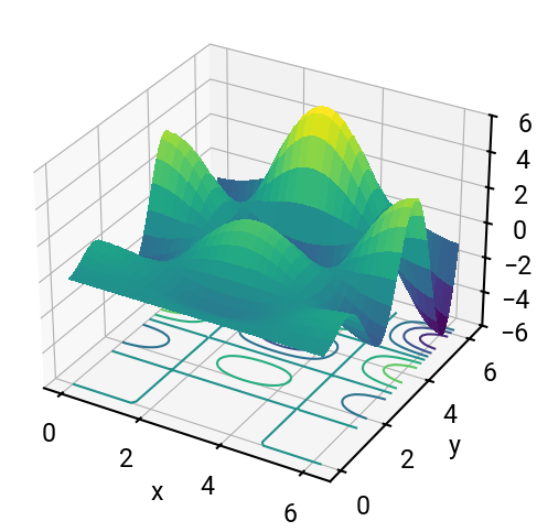
What happens if we didn’t include the offset keyword? ⛰️

Part (b)

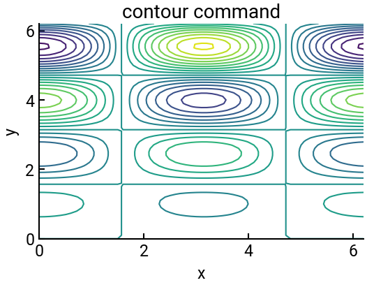
Make a 2D contour plot of the above using the ax.contour() function. This will only display the level curves in a horizontal plane, and you should verify that it is consistent with the previous plot. Include labels and a title.

Note: Using the contour command, you can specify the number of levels you would like to be displayed.

fig, ax = plt.subplots()   # now back to 2D!
ax.contour(X, Y, Z, linewidths=1.5, levels=20)
ax.set(xlabel='x', ylabel='y', title="contour command")
plt.show()