The tl;dr Python speedrun#
Note
Click the and open this notebook in Colab to enable interactivity.
Note
To save your progress, make a copy of this notebook in Colab File > Save a copy in Drive and you’ll find it in My Drive > Colab Notebooks.
Part of the MATLAB tutorials in CME 100 features a condensed set of notes, which we’ve reproduced here in Python.
1. Basic operations#
(a) Using Python as a calculator#
You can always type numerical expressions and perform a direct computation.
(2 + 3) * 4 / 5
4.0
(b) Defining scalar variables#
This is done with the = assignment operator.
variable_name = value.
a = 2
a
2
b = 3
b
3
c = a + b
c
5
# this is a comment
c;    # semicolon suppresses output
(c) Defining arrays and using array elements in computation#
🚨 Remember that Python is 0-indexed!
Otherwise the syntax is array[i] to grab the element at the \(i\)th index.
a = [1, 2, 3]
print(a)
print(a[0])
print(a[1])
print(a[2])

x = a[0] * a[1]
print(x)
[1, 2, 3]
1
2
3
2
(d) Appending arrays#
# in native Python with lists
a = [1, 2, 3]
b = [3, 4]
c = a + b
print(c)

# in NumPy with NumPy arrays
import numpy as np
a = np.array([1, 2, 3])
b = np.array([3, 4])
c = np.concatenate([a, b])
print(c)
[1, 2, 3, 3, 4]
[1 2 3 3 4]
2. Plotting#
This is done with the powerful Matplotlib library.
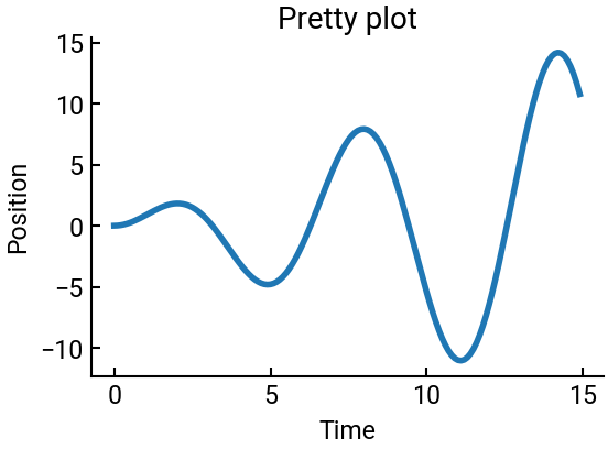
(a) Basic plotting#
import numpy as np
import matplotlib.pyplot as plt

x = np.arange(0, 15, 0.1)
y = np.sin(x) * x

fig, ax = plt.subplots()
ax.plot(x, y)
ax.set(xlabel="Time", ylabel="Position", title="Pretty plot")
plt.show()
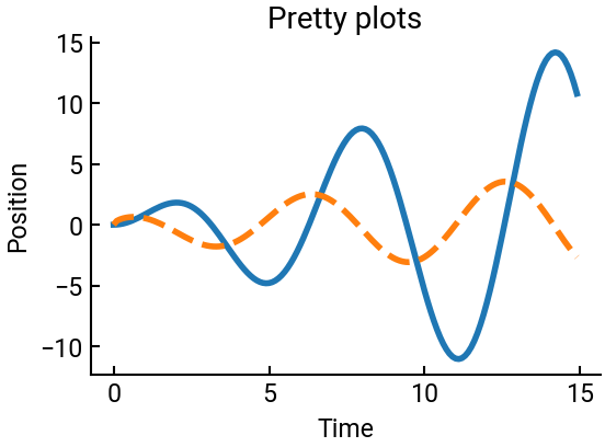
We can easily plot multiple datasets on a single set of axes.
z = np.cos(x) * x ** 0.5

fig, ax = plt.subplots()
ax.plot(x, y)
ax.plot(x, z, ls='--')
ax.set(xlabel="Time", ylabel="Position", title="Pretty plots")
plt.show()
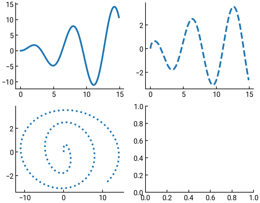
Or we can put them on separate axes on the same figure.
fig, ax = plt.subplots(figsize=(10,8), nrows=2, ncols=2)
ax[0,0].plot(x, y)
ax[0,1].plot(x, z, ls='--')
ax[1,0].plot(y, z, ls=':')
plt.show()
3. Plotting in 3D#
This is still done in Matplotlib, but with some special function parameters.
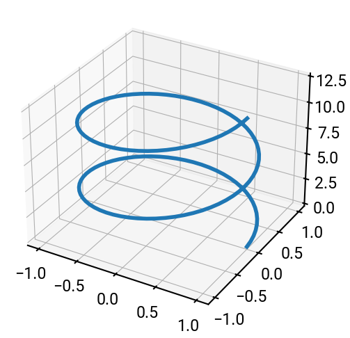
(a) Parametric curves#
import numpy as np
import matplotlib.pyplot as plt

t = np.arange(0, 4*np.pi, 0.1)
x = np.cos(t)
y = np.sin(t)
z = t

fig = plt.figure(figsize=(6,6))
ax = fig.add_subplot(projection='3d')
ax.plot(x, y, z)
plt.show()
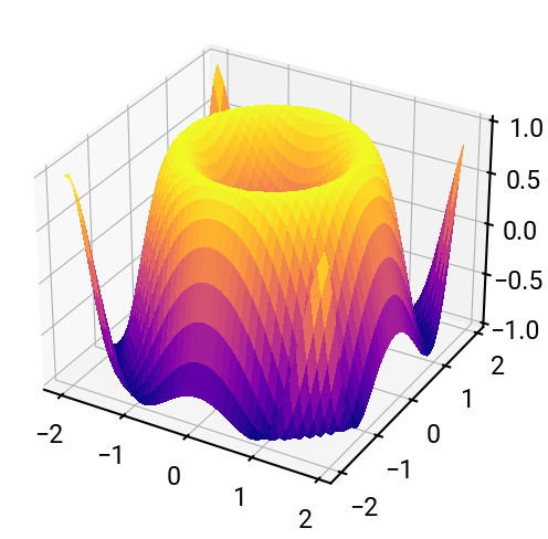
(b) Surfaces#
import numpy as np
X, Y = np.meshgrid(np.arange(-2, 2, 0.1), np.arange(-2, 2, 0.1))
Z = np.sin(X ** 2 + Y ** 2)

fig = plt.figure(figsize=(6,6))
ax = fig.add_subplot(projection='3d')
ax.plot_surface(X, Y, Z, cmap='plasma', antialiased=False)
plt.show()
4. Creating a simple script#
PASS
5. Creating a function#
The general syntax is:
def my_function(args):
    # do something
    return a_value   # optional
def dot_product(a, b):
    return a[0] * b[0] + a[1] * b[1] + a[2] * b[2]

a = [1, 2, 3]
b = [2, 3, 4]
dot_product(a, b)
20
6. Using functions#
Where we use the function from the previous cell.
import numpy as np
a = [1, 2, 3]
b = [2, 3, 4]
c = dot_product(a, b)
proj_ab = c / np.linalg.norm(b)
print(c, proj_ab)
20 3.7139067635410377
7. Programming in Python#
As with most problems, there are multiple possible solutions, and the idea is we pick the one that is most logical and/or efficient.
def factorial_for(n):
    product = 1
    for i in range(2, n+1):
        product *= i
    return product

def factorial_while(n):
    product = 1
    i = 1
    while i <= n:
        product *= i
        i += 1
    return product

def factorial_if(n):
    product = 1
    i = 1
    while True:
        product *= i
        i += 1
        if i > n:
            break
    return product

print(factorial_for(8), factorial_while(8), factorial_if(8))
40320 40320 40320
Conclusion#
Congrats on making it to the end of this accelerated tutorial!