14. Surfaces in 3D

Now that we’re familiar with 1D plots, it’s time to move on to 3D visualizations!

Summary of commands

In this exercise, we will demonstrate the following:

• np.meshgrid(x, y) - Create a 2D grid of coordinate values based on 1D x and y arrays.

  • The result is two X and Y 2D arrays with the corresponding 1D arrays tiled across the other dimension.

• fig.add_subplot(projection='3d') - A common way of creating 3D axes.

• ax.plot_surface(X, Y, Z) - Create a 3D surface plot of Z on the domain defined by meshgrid X and Y.

• fig.colorbar(obj) - Add a color bar corresponding to the obj plot element.

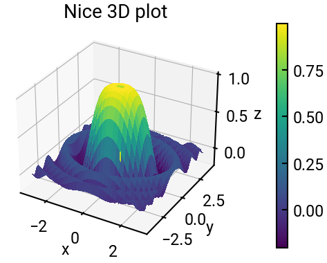
We will plot the function

\[ z(x,y) = \dfrac{\sin(x^2 + y^2)}{x^2 + y^2 + 10^{-16}} \]

for \(x\) ranging between \(-3\) and \(3\), and \(y\) ranging between \(-4\) and \(4\). Use an increment of \(0.1\) in both directions. Include labels and a title, and add a color bar to the figure.

Note

The \(10^{-16}\) in the denominator is needed to avoid division by zero when \(x = y = 0\). Some sources may write this as \(\varepsilon\) (Greek letter epsilon) to represent a tiny quantity.

import numpy as np
import matplotlib.pyplot as plt

# values
x = np.arange(-3, 3, 0.1)
y = np.arange(-4, 4, 0.1)
X, Y = np.meshgrid(x, y)
print(X.shape)
Z = np.sin(X**2 + Y**2) / (X**2 + Y**2 + 1e-16)

fig = plt.figure(figsize=(6,6))
ax = fig.add_subplot(projection='3d')
surf = ax.plot_surface(X, Y, Z, cmap='viridis', antialiased=False)
fig.colorbar(surf, pad=0.15, shrink=0.7)
ax.set(xlabel='x', ylabel='y', zlabel='z', title='Nice 3D plot')
plt.show()

(80, 60)

Several things to note

Meshgrid

• Look at the shape of \(X\) (or \(Y\), \(Z\)): It is two dimensional, and if you look the values, it essentially repeats every value of \(x\) at every value of \(y\) (and vice versa).

• A lesson in descriptive variable names: In math, we are used to using lowercase letters for scalars/vectors, and uppercase letters for matrices. So we do the same here!

Surface plot

• We used the cmap parameter when making the surface plot to choose an appropriate colormap. Otherwise the whole plot is a default blue and less helpful.

• We also added antialiased=False which is somewhat similar to shading('interp') that you might be used to seeing in MATLAB.

• We did not modify the rstride and cstride parameters, but you could to make the rendering finer (e.g., set both to 1).

Other

• We had to tweak the color bar a little bit to make it fit better. See the documentation for more details.

• We might not get the nice click-and-drag features of MATLAB plots in Colab (there are other interactive plotting libraries), but if you wanted to change the viewing angle, you can explore ax.view_init(elev, azim, roll).