T2: Control flow

T2: Control flow#

Note

Click the and open this notebook in Colab to enable interactivity.

Note

To save your progress, make a copy of this notebook in Colab File > Save a copy in Drive and you’ll find it in My Drive > Colab Notebooks.

This week we are covering control flow, which is a broad term that describes statements that determine the order of code execution and the direction your program will take based on certain conditions being met (or not). Mastering control flow will make your code more efficient and effective!

Conditional statements#

We use this to describe if, elif (short for “else if”), and else statements. The general structure is like this:

if condition1:
    <do something only when condition1 is True>
elif condition2:
    <otherwise, do something else if condition2 is True> (and condition1 was False)
else:
    <otherwise, do something else>

Note

if is required, and the other two are optional.

Note

In MATLAB, control flow blocks have an end to conclude. No need for that in Python!

Here is an example:

x = 5
y = 0
if x > 0:
    y = 1
y

Check: If you change the first line to x = 0, what will appear when you run it again?

The statement y = 1 will be executed if x > 0 evaluates to True. We can tell Python to do something else when x > 0 evaluates to False by using elif and else.

x = 5
y = 0
if x > 0:
    y = 1
elif x < 0:
    y = -1
else:
    y = 0

y

Check: Change the value of x several times with positive, negative, and zero values and run the previous cell again.

Finally, take a look at this:

a = 2
b = 4
if a == 2 and b == 4:
    print("wow!")

wow!

Important

In Python, logical “and” uses the actual word and instead of the symbols && as it’s commonly done in other languages. Similarly, logical “or” uses the actual word or. Finally, please don’t confuse these keywords (no quotes) with the literal strings 'and' and 'or'!

Self-referencing assignments (optional)#

Self-referencing assignment is the idea of updating a variable to a new value using its current (old) value. Try to do the following:

Create variable x with value 0. Then type x = x + 1.
Type x = x + 1 again.
Type x = x + 1 again.
Print x. What do you expect to see?
Create variable y with value 1. Then type y = y * x.
Type y = y * x again.
Type y = y * x again.
Print y. What do you expect to see?

# TODO: Write your solution below

Loops#

Loops are one of the main advantages of a programmatic solution, as they enable you to automate repetitive tasks.

For loops#

A for loop is used to repeat execution of a chunk of code when you know how many times you will repeat. In many applications, for loops are used in combination with self-referencing assignments.

The for loop syntax in Python is:

for i in collection:
    <do something repeatedly, where each iteration, the variable i takes on a different value in the collection>

where collection is usually a list-like object of values. The for loop stops when all the items in the collection are used once. A very common expression you’ll see for collection is range(N), which is a built-in function that enumerates numbers from 0 up to N (not inclusive).

The full function signature is range(start, stop, step), going from start to stop (not inclusive) in steps of size step.

s = 0
for i in range(1, 11):
    s = s + i
s

# change s to a list and grow it
s = [0]
for i in range(1, 11):
    s.append(s[-1] + i)
s

[0, 1, 3, 6, 10, 15, 21, 28, 36, 45, 55]

# change the step size
s = 0
for i in range(1, 20, 2):
    s = s + i
s

There are numerous applications of for loops. For now, we will discuss how to plot a function that has different definitions on different pieces of the domain. This example demonstrates the use of if and for together.

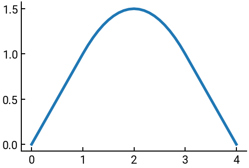
Example#

Plot the function \(f(x)\) defined by

\[\begin{split} f(x) = \begin{cases} x & 0 \le x \le 1 \\ \dfrac{3}{2} - \dfrac{1}{2} (x - 2)^2 & 1 \le x \le 3 \\ 4 - x & 3 \le x \end{cases}, \end{split}\]

over the domain \(x \in [0, 4]\) with step size \(\Delta x = 0.1\).

Consider:

Should you use np.arange() or np.linspace() to create x?
You should first preallocate y (the array for \(f(x)\)) by using np.zeros(shape) to create a \(\vec{0}\)-vector of the same shape as x.

# import libraries
import numpy as np
import matplotlib.pyplot as plt

# discretize the domain in equal steps
x = np.arange(0, 4.1, 0.1)

# initialize y
y = np.zeros(x.shape)

# using a for loop to compute y at each value of x
for i in range(len(x)):
    if x[i] <= 1:
        y[i] = x[i]
    elif x[i] <= 3:   # we don't need the "other side" because it's already handled
        y[i] = 3/2 - 1/2 * (x[i] - 2)**2
    else:
        y[i] = 4 - x[i]

# we plot the result
fig, ax = plt.subplots()
ax.plot(x, y)
plt.show()

../_images/26da6eefb54a39c68879e53a68e686d43b4c8889b59e607c0dfa159169077c69.png

While loops#

A while loop is, in a sense, similar to an if statement, but the execution will be repeated until the condition no longer holds. In other words, it’s a loop where you know the stop condition, but you don’t know (or don’t care) how many iterations it will take to get there.

The while loop syntax in Python is:

while condition:
    <do something repeatedly until condition becomes False>
    # Try not to get stuck in an infinite loop!

Example#

Find a solution to the equation \(x = \cos x\) with error not greater than \(0.01\).

Idea: If \(x\) is a solution to the equation, then applying \(\cos\) to \(x\) would not change the value. We hope that if we start with an arbitrary number and repeatedly apply \(\cos\), we will eventually get (very close) to the solution of \(x = \cos x\). (The reason why this works, known as fixed-point iteration, is beyond the scope of this class.)

# pick an abitrary number to start from, say 1
x = 1

# repeat until |x - cos(x)| < 0.01
while np.absolute(x - np.cos(x)) >= 0.01:
    x = np.cos(x)
print(x)
print(np.absolute(x - np.cos(x)))

0.7442373549005569
0.008632614464209598

Note

Look carefully at the condition following the keyword while. It is the negation of the terminating condition.

For vs. While#

If you know the number of iterations in advance, it is a good practice to use for.

Example#

Compute the first \(25\) Fibonacci numbers.

# initialize
fibo = [1, 1]
for i in range(2, 25):
    fibo.append(fibo[i - 1] + fibo[i - 2])
fibo

When the number of iterations is not known in advance, we can only use while.

Example#

Compute all Fibonacci numbers that are not greater than \(10,000,000\).

fibo = [1, 1]
while fibo[-1] <= 1e7:
    fibo.append(fibo[-1] + fibo[-2])
fibo   # overcounts one, but we'll ignore it

Logical operations (optional)#

The “conditions” used in for and while statements are logical expressions. Here’s how they work in more detail.

Two vectors of the same dimension can be compared. The result is a vector of truth values (0 and 1) of the same dimension. Available comparison operators are

== (equal to)
!= (not equal to)
> (greater than)
>= (not smaller than)
< (smaller than)
<= (not greater than).

Try the following commands:

print(4 > 2)
print(4 < 2)

a = np.array([1, 2, 3, 4, 5])   # would not work with pure lists!
b = np.array([2, 2, 2, 4, 4])
print(a == b)

print(np.arange(10, 0, -1) >= np.arange(10))

True
False
[False  True False  True False]
[ True  True  True  True  True  True False False False False]

These comparison operators work entrywise, so scalar expansion will happen when one of the two operands is a scalar.

print(np.arange(-3, 3) < 0)
print(np.arange(10) != 5)

[ True  True  True False False False]
[ True  True  True  True  True False  True  True  True  True]

The above comparison are often used to create masks of logical indices for selecting a subset of an array.

There are also element-wise logical connectives in Python, such as np.logical_and(x, y) and np.logical_or(x, y). 0 is considered False while all non-zero numbers are considered True.

a = np.array([0, 0, 1, 1])
b = np.array([0, 1, 0, 1])

print(np.logical_and(a, b))
print(np.logical_or(a, b))

[False False False  True]
[False  True  True  True]

T2: Control flow

Contents

T2: Control flow#

Conditional statements#

Self-referencing assignments (optional)#

Loops#

For loops#

Example#

While loops#

Example#

For vs. While#

Example#

Example#

Logical operations (optional)#