T1: Fundamentals and plotting

Note

Click the and open this notebook in Colab to enable interactivity.

Note

To save your progress, make a copy of this notebook in Colab File > Save a copy and you’ll find it in My Drive > Colab Notebooks.

Previously in this book we’ve already motivated the use of Python, so in this first tutorial we’ll jump right into its functionality!

Performing calculations

We can use Python as a calculator, with the following operators:

• +: addition

• -: subtraction

• *: multiplication

• /: division

• **: exponentiation.

Try computing \(\sqrt{3^2 + 4^2}\) below. Recall that \(\sqrt{x} = x^{1/2}\).

# TODO: Write your solution below

Decimals (the float type in Python) can be input like normal or as scientific notation.

print(0.0041)
print(4.1e-3)

0.0041
0.0041

Since Python was not developed for scientific computing, it doesn’t have built-in functions and constants. But it has many freely available packages that do, including the popular NumPy library. To import the library, we use the

import numpy as np

syntax to give it an alias, and then we can call functions and constants from the np namespace. Below we will compute

\[ \sqrt{1 - \sin^2 \left( \frac{2}{3} \pi \right)} \]

using the functions np.sqrt(), np.sin(), and the constant np.pi.

# TODO: Write your solution below

Results of computation can be stored in variables by using the assignment operator, = (not for checking equality!). For example, x = 5.2 would create a variable named x and store 5.2 in it. If x already exists, x = 5.2 will replace the old value in x with 5.2, even if the old value wasn’t a decimal! After a variable is made, it can be used in other expressions.

In the cell below, define a variable that holds the value of \(\sqrt{2 \pi e}\) and use it to compute

\[ \frac{1}{\sqrt{2\pi e}} e^{\sqrt{\frac{2}{\pi e}}} + \sqrt{2 \pi e} \]

where \(e\) is Euler’s constant np.e and \(e^x\) is encoded as np.exp().

# TODO: Write your solution below

Creating variables reduces the amount of calculation (and coding) at the cost of additional memory. This speed-memory trade-off is very common in programming.

Note

A variable name must start with an English alphabet and may only contain letters, numbers, and underscores (_). It is also Python style to write variable names in snake case, lowercase_like_this.

Arrays and vectors

To create a row vector in Python, we will use brackets and commas to first create a list data structure, and then use the np.array() constructor.

To read from an entry of a vector in a variable, we use square brackets and the index. For example: x[1] refers to the second entry of array x.

Important

Python is 0-indexed which means the first element of an array is array[0], not 1! This is one of the biggest differences between Python and MATLAB.

Below we will assign \(\begin{bmatrix} 1 & 2 & 3 \end{bmatrix}\) to x and then read out the second entry of x.

# TODO: Write your solution below

Assignment to an entry of a vector also works. If the referenced entry of a vector does not exist, Python will throw an error.

import numpy as np
x = np.array([1, 2, 3])
x[2] = 5
x[3] = 0

---------------------------------------------------------------------------
IndexError                                Traceback (most recent call last)
Cell In[6], line 4
      2 x = np.array([1, 2, 3])
      3 x[2] = 5
----> 4 x[3] = 0

IndexError: index 3 is out of bounds for axis 0 with size 3

There are some helper functions that make it easier to create vectors, depending on your need. A detailed exposition is provided in the docs.

I want exactly \(N\) equally spaced values

Here you want to use the np.linspace(start, stop, num) function, which accepts as arguments:

• start: The first value of your array. Required.

• stop: The last value of your array. Required.

• num: The total number of elements in your array, equally spaced between start and stop inclusive (by default). If you do not specify this parameter, the default is num=50.

I want values equally spaced by \(\delta\)

Here you want to use the np.arange(start, stop, step) function, which accepts as arguments:

• start: The first value of your array. Default is 0, but best to always specify.

• stop: The last value of your array, not inclusive. Required.

• step: The increment between values starting from start and going up to but not including stop. Default is 1, but best to always specify.

Try it now with the following:

• np.linspace(1, 9, 4)

• np.arange(1, 2.5, 9)

# TODO: Write your solution below

We can use the len() function to get the length of an array. We can also use the built-in array.size attribute.

arr = np.arange(7, 60, 7)    # [7, 14, ..., 56]
print(len(arr))
print(arr.size)

8
8

Operations on arrays

NumPy arrays of the same dimension can be added and subtracted. Don’t try this with basic lists!

a = np.array([1, 2])
b = np.array([4, 5])
c = np.array([4, 5, 6])
print(a - b)
print(a - c)

[-3 -3]

---------------------------------------------------------------------------
ValueError                                Traceback (most recent call last)
Cell In[9], line 5
      3 c = np.array([4, 5, 6])
      4 print(a - b)
----> 5 print(a - c)

ValueError: operands could not be broadcast together with shapes (2,) (3,) 

Multiplication, division, and exponentiation between two vectors of the same dimension can be performed entrywise using the standard operators. Try it below for [4, 3] raised to the power of [0.5, 2].

# TODO: Write your solution below

A vector with one element is considered a scalar. Entrywise operations between a scalar and a vector will cause scalar expansion, also known as array broadcasting. This can be a good thing, but often it isn’t!

# first example - comparison
print(1 + np.array([2, 3]))
print(np.array([1, 1]) + np.array([2, 3]))

# second example
print(np.arange(11) ** 2)

# third example
print(((-1) ** np.arange(1, 7) + 1) / 2)

[3 4]
[3 4]
[  0   1   4   9  16  25  36  49  64  81 100]
[0. 1. 0. 1. 0. 1.]

Scalar functions (such as those mentioned above) can be applied to a vector. They will be computed on each entry, giving the result in a vector with the same dimension as the input. Try it below with:

• np.sqrt([1, 4, 9, 16, 25]) (note it autoconverts the argument)

• np.sin(np.arange(0, 2.1, 0.5) * np.pi)

# TODO: Write your solution below

Plotting

There are many choices for plotting libraries, arguably the most popular one being Matplotlib. The name is actually a combination of “MATLAB,” “plot,” and “library,” so many things will look similar to MATLAB. Like NumPy, the documentation is quite good—and they have cheat sheets!

The general recipe of making plots with Matplotlib has four (maybe five) parts.

1. Imports

import matplotlib.pyplot as plt

is the bare minimum, other packages (like colormaps) are also possible.

2. Create objects

fig, ax = plt.subplots()

The fig Figure is the entire graph object and ax Axes is the coordinate axes. plt.subplots() is quite powerful.

3. Draw data

ax.plot(x, y)

for example, will create a standard line chart. There are many plot types available!

4. Styling (optional)

ax.set()

among other functions can add labels and customize axis features.

5. Display and save

plt.show()
fig.savefig('filename.png')

These commands go at the very end. plt.show() displays the plot in the notebook while fig.savefig() saves it to disk.

We’ll create some 2D plots in Python using ax.plot(). The first input is a vector of \(x\)-coordinates and the second input is a vector of \(y\)-coordinates. Both vectors must have the same length.

import matplotlib.pyplot as plt
fig, ax = plt.subplots()
ax.plot([0, 1, 2, 0], [1, 0, 2, 1])
ax.plot([0, 1, 2, 3, 4, 5], [0, 2, 0, 2, 0, 2])
plt.show()

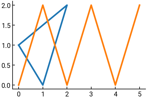
Note that unlike MATLAB, the second call to ax.plot() does not erase the previous plot. In fact, it default cycles to a different color to differentiate the two. No need for hold on!

Let’s try another plot with some customization. Type the following code:

x = np.arange(6)
y = 1 - (-1) ** x
fig, ax = plt.subplots()
ax.plot(x, y)
ax.set(xlim=[-1, 6], ylim=[-1, 3])
plt.show()

# TODO: Write your solution below

Plotting parametric curves

Take the following problem: Draw a curve in the plane parametrized by \(x(t) = t \cos t\) and \(y(t) = t \sin t\) for \(t \in [0, 6\pi]\). We could tackle the problem as follows:

1. Identify the domain of the parameter and create a vector of parameter values. We discretize the interval \([0, 6\pi]\) into 100 (or any large number) of points using t = np.linspace(0, 6*np.pi, 100).

2. Define the coordinate vectors for x and y separately, such as x = t * np.cos(t).

3. Make the plot using ax.plot(x,y).

Now, in the space below, compute the following: Draw an ellipse with major and minor radii of 2 and 1, respectively. It is parametrized by \(x(\theta) = 2 \cos \theta\) and \(y(\theta) = \sin \theta\), where \(\theta\) is the parameter.

# TODO: Write your solution below

If the output above does not look like the ellipse you’re expecting, it’s likely because the aspect ratio of the plot is not 1:1, i.e., 1 unit on the \(x\)-axis doesn’t have the same size as 1 unit on the \(y\)-axis. Use ax.set(aspect='equal') to fix this.

Further customizing plots

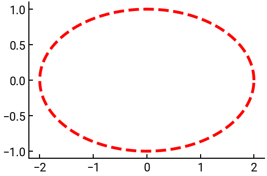
The ax.plot() command can take additional arguments to control how the plot is drawn. For example, if we had ax.plot(x, y, 'r--'), then we would get a different ellipse. Check out the documentation to see all the features.

fig, ax = plt.subplots()
t = np.linspace(0, 2 * np.pi, 1000)
x = 2 * np.cos(t)
y = np.sin(t)
ax.plot(x, y, 'r--')
plt.show()

Can you make an ellipse with a black dotted line instead?

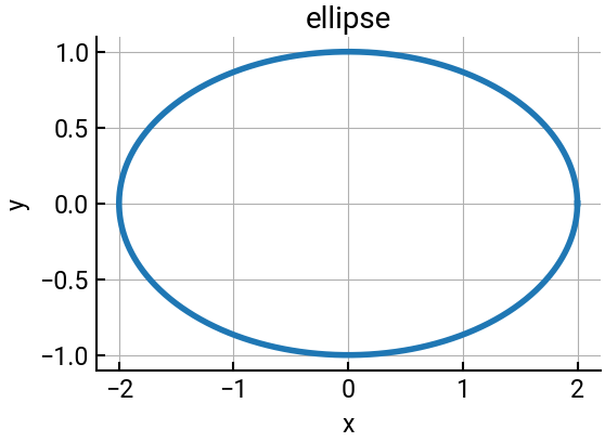
Below we give many more customization for you to explore.

fig, ax = plt.subplots()
ax.plot(x, y)
ax.set(xlabel='x', ylabel='y', title='ellipse')
ax.grid('on')
plt.show()

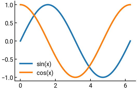
You can add legends in a couple of different ways. For now, we’ll show the syntax where you add label= as a keyword argument to ax.plot(), and call ax.legend() at the end.

x = np.linspace(0, 2* np.pi, 1000)
fig, ax = plt.subplots()
ax.plot(x, np.sin(x), label="sin(x)")
ax.plot(x, np.cos(x), label="cos(x)")
ax.legend()
plt.show()

Subplots

If you found it odd that we called plt.subplots() (plural) but only created one set of axes, well here’s how we can get more. By specifying nrows and ncols, we can get a whole grid of axes to draw on. For example, below we’ll plot on a specific subplot in a 3-by-2 grid of subplots. We’ll also make them share an \(x\)- and \(y\)-axis (they don’t have to, it makes the labels cleaner).

fig, ax = plt.subplots(nrows=3, ncols=2, sharex=True, sharey=True)
ax[1,1].plot(x, y, 'g--')
plt.show()

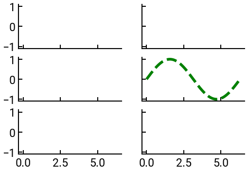
For you: Can you customize the above code to add a curve (in a different style) to another subplot?

Script files

While our commands are nicely stored in this Jupyter notebook, maybe you actually want a Python file (.py extension) to run from the command line. For the most part, you can take all the commands we’ve written them here, save them into a test.py file, and then call python test.py from the command line in the same directory.