11. Car motion example

The next few exercises in this workbook will give us a chance to practice what we’ve learned so far through engineering applications.

Newton’s laws of motion

Starting from rest, a car (mass = \(900\) kg) accelerates under the influence of a force of \(2000\) N until it reaches \(13.89\) m/s (\(50\) km/h). What is the distance traveled? How long does it take to travel this distance?

Recall that Newton’s second law of motion says:

\[ F = m \dfrac{dv}{dt} \tag{1} \]

This equation determines the velocity of the car as a function of time. To obtain the position of the car, we use the following kinematic relation:

\[ v = \dfrac{dx}{dt} \tag{2} \]

Although this problem can be solved analytically, in this exercise we would like to come up with a numerical solution using Python. We first need to discretize the equations, i.e., evaluate the position and velocity at equally spaced discrete points in time, since Python doesn’t know how to interpret continuous functions. The solution for \(v(t)\) and \(x(t)\) will then be represented by vectors containing the values of the velocity and the position of the car respectively at these discrete points in time separated by \(\Delta t\).

The time derivative for the velocity in Equation 1 can be approximated by:

\[ \dfrac{dv}{dt} \approx \dfrac{v(t + \Delta t) - v(t)}{\Delta t} \]

Equation 1 then becomes:

\[ \frac{F}{m} = \dfrac{v(t + \Delta t) - v(t)}{\Delta t} \quad \Leftrightarrow \quad v(t + \Delta t) = v(t) + \Delta t \frac{F}{m} \]

or, if we solve for the velocity at step \(n+1\):

\[ v(n+1) = v(n) + \Delta t \dfrac{F}{m} \]

where the unknown is \(v(n + 1)\).

Similarly, Equation 2 becomes:

\[ \dfrac{x(t + \Delta t) - x(t)}{\Delta t} = v(t) \quad \Leftrightarrow \quad x(t + \Delta t) = x(t) + \Delta t v(t) \]

and the position at step \(n + 1\) will be given by:

\[ x(n+1) = x(n) + \Delta t v(n) \]

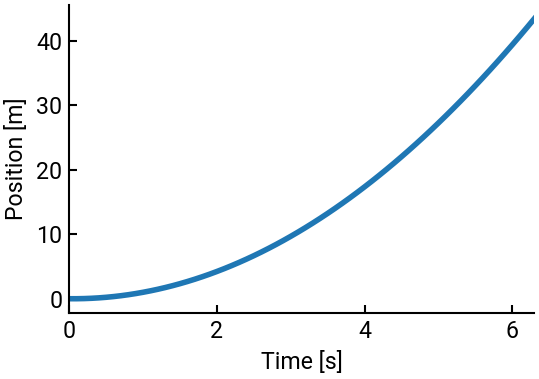
Solve the above equations for position and velocity and plot the position as a function of time. Take \(\Delta t = 0.1\) s. Display the distance traveled and the time it takes to reach \(50\) km/h.

import numpy as np
import matplotlib.pyplot as plt

F = 2000     # force in Newtons
m = 900      # mass in kilograms
dt = 0.1     # time step in seconds
vf = 13.89   # final velocity

t = [0]
v = [0]
x = [0]

while v[-1] < vf:
    t.append(t[-1] + dt)
    v.append(v[-1] + F/m * dt)
    x.append(x[-1] + v[-2] * dt)   # note the indexing since we already appended to v!

print(f"We traveled {x[-1]:.1f} m and it took {t[-1]:.1f} s!")
fig, ax = plt.subplots()
ax.plot(t, x)
ax.set(xlabel="Time [s]", ylabel="Position [m]", xlim=[0,t[-1]])   # set x-axis limits to look a bit nicer
plt.show()

We traveled 43.4 m and it took 6.3 s!

Note

Discretizing Newton’s laws of motion for computational physics seems straightforward, but it’s actually a great lesson in numerical schemes and error analysis. The above scheme, which may be called Euler’s method, is easier to understand but not very precise, as the error scales as \(\Delta t\). In Enze’s molecular dynamics simulations, for example, which propagate hundreds of thousands of atoms colliding over billions of time steps, these errors add up! There are other clever tricks scientists employ, and you’ll learn about a class of Runge-Kutta methods in CME 102!