16. Motion of a particle#
We will continue working with 3D plots, this time to visualize the 3D motion of a particle.
Summary of commands#
In this exercise, we will demonstrate the following:
np.gradient(y, x)- Computes the numerical derivative of a functionywith a spacing defined byx.np.arccos(x)- Computes the inverse cosine ofx.
The motion of a particle in three dimensions is given by the following parametric equations:
Part (a)#
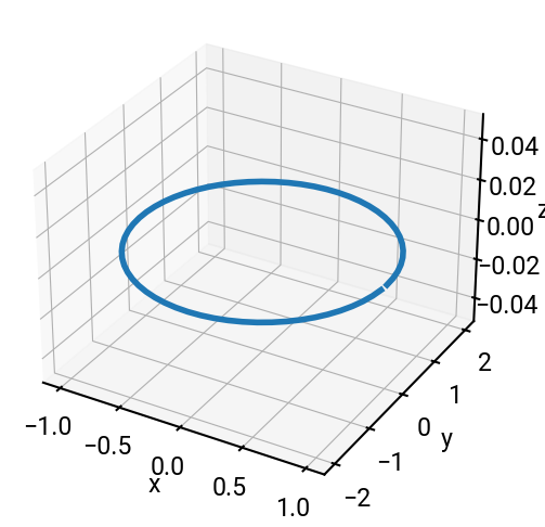
Let \(\Delta t = 0.1\).
Plot the particle’s trajectory in 3D using ax.plot().
import numpy as np
import matplotlib.pyplot as plt

# values
dt = 0.1
t = np.arange(0, 2*np.pi, dt)
x = np.cos(t)
y = 2 * np.sin(t)
z = 0 * t   # so it's the same length as the other arrays

# make a plot
fig = plt.figure(figsize=(6,6))
ax = fig.add_subplot(projection='3d')
ax.plot(x, y, z)
ax.set(xlabel='x', ylabel='y', zlabel='z')
plt.show()
Part (b)#
Compute the velocity components \(v_x\), \(v_y\) and the magnitude of the velocity vector.
vx = np.gradient(x, t)
vy = np.gradient(y, t)
speed = np.sqrt(vx**2 + vy**2)
speed
array([1.99729324, 1.98919175, 1.96689351, 1.93017098, 1.8796965 ,
       1.81643423, 1.74166731, 1.65703946, 1.56461634, 1.46697278,
       1.36730958, 1.26959233, 1.17867267, 1.10028332, 1.04069645,
       1.00579938, 0.99961014, 1.02289199, 1.07285505, 1.14419219,
       1.23064057, 1.32617291, 1.42555711, 1.52447007, 1.61941018,
       1.70755809, 1.78664863, 1.85487138, 1.91079929, 1.95333954,
       1.98170097, 1.99537336, 1.9941153 , 1.97794889, 1.94716019,
       1.90230562, 1.84422532, 1.77406565, 1.69331418, 1.60385208,
       1.50802992, 1.40877216, 1.30970904, 1.21531345, 1.13096786,
       1.06279441, 1.01699561, 0.99856397, 1.00973406, 1.04913502,
       1.11232201, 1.19325013, 1.28569147, 1.38405007, 1.48362841,
       1.58059932, 1.67187661, 1.75497841, 1.82791536, 1.88910802,
       1.93732936, 1.97166587, 1.98590301])
Part (c)#
Compute the acceleration components \(a_x\), \(a_y\) and the magnitude of the acceleration vector.
ax = np.gradient(vx, t)
ay = np.gradient(vy, t)
accel = np.sqrt(ax**2 + ay**2)
Part (d)#
Compute the components of the unit tangent vector \(\vec{T} = \begin{bmatrix} T_x & T_y & T_z \end{bmatrix}\).
Tx = vx / speed
Ty = vy / speed
Part (e)#
Compute the angle \(\theta\) between the velocity vector and the acceleration vector.
theta = np.arccos((vx * ax + vy * ay) / speed / accel)
theta
array([1.74381977, 1.78273525, 1.85495636, 1.97138039, 2.06439307,
       2.13377245, 2.18087053, 2.20727665, 2.21409273, 2.20162567,
       2.16932095, 2.11588817, 2.0397079 , 1.93972052, 1.81694275,
       1.67624376, 1.52704366, 1.38143673, 1.25034503, 1.14057129,
       1.05453971, 0.99183718, 0.95093376, 0.93033042, 0.92913875,
       0.94730482, 0.98562065, 1.04553183, 1.12861343, 1.23550156,
       1.36422403, 1.50855975, 1.65798661, 1.80033427, 1.92569072,
       2.02861905, 2.10771652, 2.16388005, 2.19872022, 2.21359787,
       2.20916979, 2.18523603, 2.1407826 , 2.07425186, 1.98420339,
       1.87057053, 1.7364322 , 1.58937576, 1.44078869, 1.30256088,
       1.18339891, 1.08742301, 1.01517252, 0.96540454, 0.9365088 ,
       0.92729992, 0.93736505, 0.9671546 , 1.01788256, 1.09116384,
       1.18819715, 1.24873431, 1.28284446])