15. Gradient

Taking derivatives is the bread and butter of calculus, so it’s time to explore how we can do so numerically.

Summary of commands

In this exercise, we will demonstrate the following:

• np.gradient(y, x) - Computes the numerical derivative of a function y with a spacing defined by x.

This function takes an input array as the first argument, and then optionally a second argument to specify the spacing between values in the first array. The default spacing is 1 (probably not what you want!) and this flexibility allows you to calculate gradients even for unevenly spaced arrays.

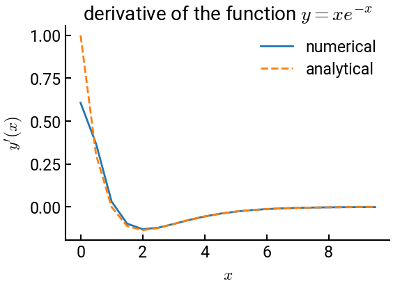
Find the derivative of the following function: \(y = xe^{-x}\) for \(x\) ranging between \(0\) and \(10\), with an increment of \(0.5\). Plot both the analytical and the numerical derivatives in the same figure.

import numpy as np
import matplotlib.pyplot as plt

# values
x = np.arange(0, 10, 0.5)
y = x * np.exp(-x)

# compute numerical and analytical gradients
grad_y = np.gradient(y, x)
dydx = (1 - x) * np.exp(-x)

# make the plots, add some LaTeX styling
fig, ax = plt.subplots()
ax.plot(x, grad_y, lw=2, label='numerical')
ax.plot(x, dydx, lw=2, ls='--', label='analytical')
ax.set(xlabel="$x$", ylabel="$y'(x)$", 
       title="derivative of the function $y = xe^{-x}$")
ax.legend()
plt.show()