T5: Optimization

Note

Click the and open this notebook in Colab to enable interactivity.

Note

To save your progress, make a copy of this notebook in Colab File > Save a copy in Drive and you’ll find it in My Drive > Colab Notebooks.

Optimization routines are used in many situations, both with and without constraints. Here we will demonstrate a few helpful functions that you can use to perform numerical optimization of functions.

Simple domain constraints

Example 1

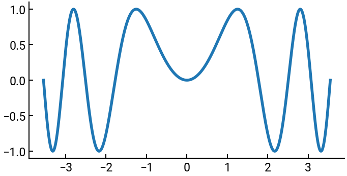
Find the local extrema of \(f(x) = \sin(x^2)\) on the interval \(\left[ -2 \sqrt{\pi}, 2 \sqrt{\pi} \right]\). Identify each point as a minimum or a maximum.

Our first solution, which isn’t exactly a solution, is to plot the function. In Python, the syntax for defining your own function is:

def my_func_name(arg1, arg2, ...):
    do something
    return something   # optional

• The def at the start is required, as is the colon at the end of the first line.

• Just like variables, function names should be descriptive.

• Arguments are optional.

• Returning a value is generally optional, but here we want to return the expression for the analytical function.

import numpy as np
import matplotlib.pyplot as plt

def my_func(x):
    return np.sin(x ** 2)

x = np.linspace(-2, 2, 1000) * np.sqrt(np.pi)

fig, ax = plt.subplots(figsize=(8,4))
ax.plot(x, my_func(x))
plt.show()

The numerical solution will leverage the fmin(func, x0) function from the scipy.optimize module. If NumPy is the library for constructing arrays, you can think of SciPy as the library that performs powerful operations on them.

You’ll notice the function signature is fmin(func, x0), where:

• x0 is your initial guess. Note that because there are many minima, we can try different guesses.

• func is an actual function (“callable”), not simply an array of numbers! This means we need a function that returns the appropriate computation on \(x\), like what we wrote above.

from scipy.optimize import fmin

fmin(my_func, 2)   # try with some different values based on the plot

Optimization terminated successfully.
         Current function value: -1.000000
         Iterations: 12
         Function evaluations: 24

array([2.17080078])

Example 2

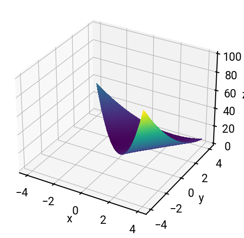
Determine the domain of \(f(x,y) = (x - y + 2)^2 + \sqrt{x + y}\) and find the global minimum.

The domain of \(f(x,y)\) is \(\{(x,y) \mid x + y \ge 0\}\). If we want to be very careful, we could mask the arrays to exclude prohibited values; or we can be lazy (Enze is lazy) and let Python gracefully handle the errors.

For this 3D function, we will use np.meshgrid(x, y) to construct a 2D grid for the domain. Then we will use ax.plot_surface(X, Y, Z) to plot the surface of Z above the domain defined by X and Y. Pay attention to how we constructed the 3D axes!

x = np.linspace(-4, 4, 1000)
X, Y = np.meshgrid(x, x)
Z = (X - Y + 2) ** 2 + np.sqrt(X + Y)

fig = plt.figure(figsize=(6,6))         # this is different! 
ax = fig.add_subplot(projection='3d')   # this is different!
ax.plot_surface(X, Y, Z, cmap='viridis', antialiased=False)
ax.set(xlabel='x', ylabel='y', zlabel='z')
plt.show()

C:\Users\enzec\AppData\Local\Temp\ipykernel_14172\3338264623.py:3: RuntimeWarning: invalid value encountered in sqrt
  Z = (X - Y + 2) ** 2 + np.sqrt(X + Y)

A few notes

• We used the cmap parameter when making the surface plot to choose an appropriate colormap. Otherwise the whole plot is a default blue and less helpful.

• We also added antialiased=False which is somewhat similar to shading('interp') that you might be used to seeing in MATLAB.

Numerical optimization

Using fmin() may not produce an accurate result in this case because the minimum is on the boundary. But we can try!

Note that fmin() can be quirky. If you have two variables x and y, instead of inputting them as separate arguments in the function, instead group them into a list, i.e., u = [x, y]. Then your x0 will be a list as well for the initial guesses.

def my_func_2D(u):
    return (u[0] - u[1] + 2) ** 2 + np.sqrt(u[0] + u[1])

fmin(my_func_2D, [1, 1])

Optimization terminated successfully.
         Current function value: 0.000026
         Iterations: 85
         Function evaluations: 161

C:\Users\enzec\AppData\Local\Temp\ipykernel_14172\2150192953.py:2: RuntimeWarning: invalid value encountered in sqrt
  return (u[0] - u[1] + 2) ** 2 + np.sqrt(u[0] + u[1])

array([-0.99993308,  0.99993309])

More complicated equality constraints

Find the minima of \(f(x, y, z) = |x^3| + |y^3| + |z^3|\) with respect to the constraint \(x^2 + y^2 + z^2 = 1\) using the method of Lagrange multipliers.

Let’s try to plot it first (once you’ve obtained the analytical solution). Note below we’ve employed the change of coordinates

• \(x = \cos \alpha \cos \theta\)

• \(y = \cos \alpha \sin \theta\)

• \(z = \sin \alpha\)

import numpy as np
import matplotlib.pyplot as plt

alpha = np.linspace(-np.pi/2, np.pi/2, 1000)
theta = np.linspace(-np.pi, np.pi, 1000)
A, T = np.meshgrid(alpha, theta)
X = np.cos(A) * np.cos(T)
Y = np.cos(A) * np.sin(T)
Z = np.sin(A)
C = np.absolute(X**3) + np.absolute(Y**3) + np.absolute(Z**3)
print(np.min(C))

fig = plt.figure(figsize=(6,6))
ax = fig.add_subplot(projection='3d')
surf = ax.plot_surface(X, Y, Z, cmap='viridis', antialiased=False)
fig.colorbar(surf, pad=0.15, shrink=0.7)
ax.set(xlabel='x', ylabel='y', zlabel='z')
plt.show()

0.5773510310689911

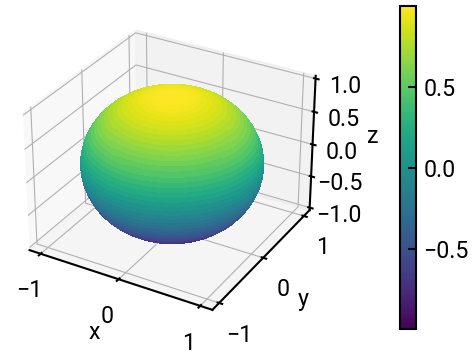
Fascinating! It’s a ball!

Let’s now try to minimize this function using fmin() and a bit of creativity… 💭

def my_func(x):
    return np.absolute(x[0]**3) + np.absolute(x[1]**3) + np.absolute(x[2]**3)

def spherical(c):
    return np.cos(c[0]) * np.cos(c[1]), np.cos(c[0]) * np.sin(c[1]), np.sin(c[0])

def combo(c):
    return my_func(spherical(c))   # nested functions!

minimizer = fmin(combo, [0, 0])
display(minimizer)

print(combo(minimizer))       # this is the minimum value

Optimization terminated successfully.
         Current function value: 0.577350
         Iterations: 73
         Function evaluations: 139

array([0.6155247 , 0.78542185])

0.5773502712665773