.ipynb .pdf

repository open issue suggest edit

JupyterHub Colab

Contents

Review of matminer features

Authors: Enze Chen and Mark Asta (University of California, Berkeley)

Note

This is an interactive exercise, so you will want to click the and open the notebook in DataHub (or Colab for non-UCB students).

Learning objectives

This notebook contains a series of exercises that review the matminer package for generating features in an automated way. By the end of this notebook, you should be able to:

1. Generate features from the chemical formula.

2. Generate features from the crystal structure.

We will rely on the matminer package for implementing these algorithms.

Contents

1. Chemical formula features

2. Crystal structure features

Motivation

So far, it sounds like everyone is off to a good start and thinking deeply about what properties might exhibit correlations with the dielectric constant \(\varepsilon\). This is a really important step at the beginning of any data-driven pipeline and it’s good practice for you to assemble the code infrastructure for a few manual cases before jumping into an automated approach.

That being said, you’re probably running out of materials properties that are present “by default” in MP, so it’s time to think about what new features we can generate (also called feature engineering) from the data that is there. We want these features to be physically meaningful, so we’ll take a look at the chemical formula and crystal structure and how we can use featurizers from matminer to convert these objects into new features.

Import Python packages

import numpy as np
import pandas as pd
pd.set_option('display.max_columns', None)
pd.set_option('display.max_rows', 300)
import matplotlib.pyplot as plt
%matplotlib inline

from sklearn.linear_model import LinearRegression
from sklearn.preprocessing import StandardScaler
from sklearn.metrics import mean_squared_error, mean_absolute_error
from sklearn.model_selection import KFold, cross_val_score, cross_val_predict

plt.rcParams.update({'figure.figsize':(8,6),       # Increase figure size
                     'font.size':20,               # Increase font size
                     'mathtext.fontset':'cm',      # Change math font to Computer Modern
                     'mathtext.rm':'serif',        # Documentation recommended follow-up
                     'lines.linewidth':5,          # Thicker plot lines
                     'lines.markersize':12,        # Larger plot points
                     'axes.linewidth':2,           # Thicker axes lines (but not too thick)
                     'xtick.major.size':8,         # Make the x-ticks longer (our plot is larger!)
                     'xtick.major.width':2,        # Make the x-ticks wider
                     'ytick.major.size':8,         # Ditto for y-ticks
                     'ytick.major.width':2,        # Ditto for y-ticks
                     'xtick.direction':'in', 
                     'ytick.direction':'in'})

### Load in your MP API key
api_key = None
try:       # this is for running locally
    import os
    api_key = os.environ['MAPI_KEY']
except:    # this is for running on DataHub
    with open('../../assets/files/mp_api_key.txt', 'r') as f:
        api_key = f.readlines()[1].strip()

# assert helps catch potential bugs
assert api_key is not None, 'API key not set correctly in environment!'
assert api_key != '', 'API key not found in mp_api_key.txt file!'

Step 1: Fetch and organize the data

We haven’t shown mechanical properties much love in this module, so let’s run a MAPI query for the elastic constants, focusing on the bulk modulus \(K\) in particular.

from pymatgen.ext.matproj import MPRester

# run the query
with MPRester(api_key) as mpr:
    entries = mpr.query(criteria={'nelements': 2,   # this is just to keep the dataset small
                                  'e_above_hull': {'$lte': 0.01}, 
                                  'elasticity': {'$exists': True}},
                        properties=['pretty_formula', 'structure', 'elasticity'])

# format data from JSON to DataFrame (tabular) --- hopefully this block looks familiar!
formulas = []
structures = []   # we'll use this later
bulk_mod = []
for entry in entries:
    formulas.append(entry['pretty_formula'])
    structures.append(entry['structure'])
    bulk_mod.append(entry['elasticity']['K_VRH'])

df = pd.DataFrame({
    'formula': formulas,
    'structure': structures,
    'bulk_modulus': bulk_mod
})
df.head()

	formula	structure	bulk_modulus
0	LiB	[[2.006491 1.15845065 0.778837 ] Li, [ 2.00...	69.0
1	LaAu	[[ 1.996426 -4.2278122 3.64861125] La, [1....	65.0
2	HoAu	[[ 1.84639 -3.95945375 3.50895675] Ho, [1....	89.0
3	FeB	[[ 1.445942 -2.6912304 2.21855775] Fe, [1....	239.0
4	DyAu	[[ 1.857119 -3.97289882 3.52320225] Dy, [1....	87.0

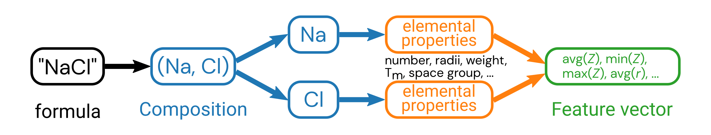
Chemical formula features

Back to top

The first featurizer we’ll discuss, which is a review of the “Featurization” notebook, is the composition featurizer, which generates chemical features from the chemical formula. We will specifically showcase the ElementProperty class, and this time do it with a little more granularity so you can pick the features that are important to you.

The procedure is as follows:

1. Perform a MAPI query using Pymatgen to fetch data (we’ve done this already).

2. Convert the chemical formula from str to a Pymatgen Composition object in a new column.

3. Construct an ElementProperty() object that specifies which new features to generate.

4. Use the featurize_dataframe() method to generate many new columns in the DataFrame, one for each feature.

Step 2: str to Composition

from matminer.featurizers.conversions import StrToComposition

# create an object for converting formula --> Composition
str_to_comp = StrToComposition(target_col_id='composition')

# perform the conversion and add a new column to the DataFrame
df_comp = str_to_comp.featurize_dataframe(df, col_id='formula')

# show the results
df_comp.head()

	formula	structure	bulk_modulus	composition
0	LiB	[[2.006491 1.15845065 0.778837 ] Li, [ 2.00...	69.0	(Li, B)
1	LaAu	[[ 1.996426 -4.2278122 3.64861125] La, [1....	65.0	(La, Au)
2	HoAu	[[ 1.84639 -3.95945375 3.50895675] Ho, [1....	89.0	(Ho, Au)
3	FeB	[[ 1.445942 -2.6912304 2.21855775] Fe, [1....	239.0	(Fe, B)
4	DyAu	[[ 1.857119 -3.97289882 3.52320225] Dy, [1....	87.0	(Dy, Au)

Steps 3 and 4: Composition to FEATURES 💥

Note that these chemical formulas all have two elements in them, so it’s not so intuitive what information to extract from the elements in this formula. Pay attention to how we are specifying the Magpie elemental features (original paper). Remember what this is doing is taking the property (such as AtomicWeight or MeltingT) of all of the constituent elements and calculating an average, maximum, minimum, etc. and using these statistical quantities of elemental properties as features. There are more composition featurizers you can try, which will be left as an exercise to the reader.

Pause and reflect: Why do we calculate statistical quantities of the individual elemental features?

from matminer.featurizers.composition import ElementProperty

# these are all the Magpie features. You can choose fewer if you want.
features = ['Number', 'MendeleevNumber', 'AtomicWeight', 'MeltingT', 
            'Column', 'Row', 'CovalentRadius', 'Electronegativity', 
            'NsValence', 'NpValence', 'NdValence', 'NfValence', 'NValence', 
            'NsUnfilled', 'NpUnfilled', 'NdUnfilled', 'NfUnfilled', 'NUnfilled', 
            'GSvolume_pa', 'GSbandgap', 'GSmagmom', 'SpaceGroupNumber']

# these are the statistical quantities we can compute
stats = ['mean']   # we can also add 'minimum', 'maximum', 'range', 'avg_dev', 'mode'

featurizer = ElementProperty(data_source='magpie',
                             features=features,
                             stats=stats)
# featurizer = ElementProperty.from_preset('magpie')   # this is what we had last time

# generate the features
df_features = featurizer.featurize_dataframe(df_comp, col_id='composition')
feature_labels = featurizer.feature_labels()   # this extracts the ugly names; but same order as "features" up above

# see the changes
df_features.head()

	formula	structure	bulk_modulus	composition	MagpieData mean Number	MagpieData mean MendeleevNumber	MagpieData mean AtomicWeight	MagpieData mean MeltingT	MagpieData mean Column	MagpieData mean Row	MagpieData mean CovalentRadius	MagpieData mean Electronegativity	MagpieData mean NsValence	MagpieData mean NpValence	MagpieData mean NdValence	MagpieData mean NfValence	MagpieData mean NValence	MagpieData mean NsUnfilled	MagpieData mean NpUnfilled	MagpieData mean NdUnfilled	MagpieData mean NfUnfilled	MagpieData mean NUnfilled	MagpieData mean GSvolume_pa	MagpieData mean GSbandgap	MagpieData mean GSmagmom	MagpieData mean SpaceGroupNumber
0	LiB	[[2.006491 1.15845065 0.778837 ] Li, [ 2.00...	69.0	(Li, B)	4.0	36.5	8.876000	1400.845	7.0	2.0	106.0	1.510	1.5	0.5	0.0	0.0	2.0	0.5	2.5	0.0	0.0	3.0	11.882917	0.762	0.000000	197.5
1	LaAu	[[ 1.996426 -4.2278122 3.64861125] La, [1....	65.0	(La, Au)	68.0	39.5	167.936019	1265.165	7.0	6.0	171.5	1.820	1.5	0.0	5.5	7.0	14.0	0.5	0.0	4.5	0.0	5.0	26.798750	0.000	0.000000	209.5
2	HoAu	[[ 1.84639 -3.95945375 3.50895675] Ho, [1....	89.0	(Ho, Au)	73.0	49.5	180.948444	1542.165	7.0	6.0	164.0	1.885	1.5	0.0	5.0	12.5	19.0	0.5	0.0	0.0	1.5	2.0	23.716667	0.000	0.000000	209.5
3	FeB	[[ 1.445942 -2.6912304 2.21855775] Fe, [1....	239.0	(Fe, B)	15.5	63.5	33.328000	2079.500	10.5	3.0	108.0	1.935	2.0	0.5	3.0	0.0	5.5	0.0	2.5	2.0	0.0	4.5	8.951250	0.762	1.055331	197.5
4	DyAu	[[ 1.857119 -3.97289882 3.52320225] Dy, [1....	87.0	(Dy, Au)	72.5	48.5	179.733284	1511.165	7.0	6.0	164.0	1.880	1.5	0.0	5.0	12.0	18.5	0.5	0.0	0.0	2.0	2.5	23.970000	0.000	0.000000	209.5

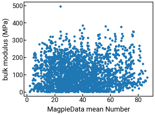
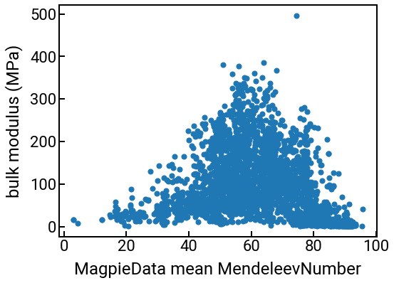
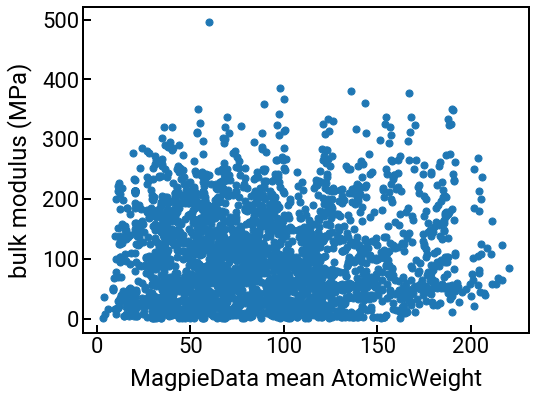
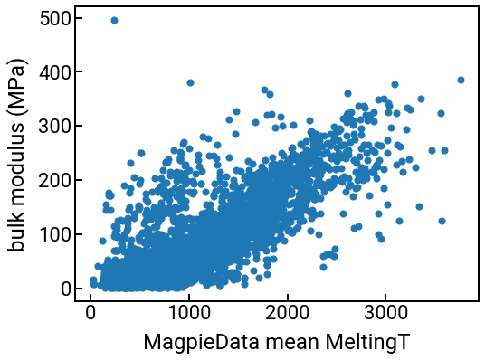
What can we do with these new features?

You can use these columns for the same things you were doing with your original features like “density” or “formation energy.” For example, we can plot them against the bulk modulus:

# we can make a series of plots in one swell foop
for i in range(4):
    single_feature = feature_labels[i]
    fig, ax = plt.subplots()
    ax.scatter(df_features[single_feature], df_features['bulk_modulus'], s=50)
    ax.set_xlabel(single_feature)
    ax.set_ylabel('bulk modulus (MPa)')
    plt.show()

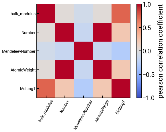
We can also compute some correlations too. Change the method in df.corr() and see what happens.

# trim the DataFrame
features_subset = ['bulk_modulus'] + feature_labels[:4]
features_subset_cleaned = [f.split()[-1] for f in features_subset]   # clean it up for plotting
df_subset = df_features[features_subset]

# construct a correlation matrix
method = 'pearson'
corr_matrix = df_subset.corr(method=method)

# plot the correlations
fig, ax = plt.subplots()
h = ax.imshow(corr_matrix, cmap='coolwarm', vmin=-1, vmax=1)   # haha you can prob choose better colors
ax.set_xticks(range(len(features_subset_cleaned)))
ax.set_xticklabels(features_subset_cleaned, rotation=60, fontsize=14)
ax.set_yticks(range(len(features_subset_cleaned)))
ax.set_yticklabels(features_subset_cleaned, fontsize=14)
plt.colorbar(h, label=f'{method} correlation coefficient')
plt.show()

We think matminer is a pretty cool package to know, and we hope it makes your lives a little bit easier.

~ BREAK ~ At this point, we highly suggest you give yourself a decent break before continuing further. 🥰 Get a drink of water, go grab a bite, or at least stand up and stretch to give your eyes a break. You all are awesome!! 🙌

Crystal structure features

Back to top

While chemistry/composition plays a big role in materials properties, we know that materials structure is important as well. After all, graphene, diamond, nanotubes, and buckyballs all have the same composition, but wildly different properties. Another material property that we get “for free” at least from MP is the crystal structure of that material, which is encoded as a Pymatgen Structure object. As we’ve already been discussing features related to crystal structure, we would like to use the structure to engineer relevant features. The procedure is very similar to how we featurized the Composition up above.

But first, let’s explore what is available in a Structure object (recall that we stored this in the structure column of our initial DataFrame after querying the MAPI).

# get the first structure for demonstration
struct = df.loc[0, 'structure']
print(struct)
print()
print(f'The density is {struct.density}')
print()
print(f'The volume is {struct.volume}')
print()
print(f'The space group is {struct.get_space_group_info()}')

Full Formula (Li2 B2)
Reduced Formula: LiB
abc   :   4.012983   4.012983   3.115348
angles:  90.000000  90.000000 120.000009
Sites (4)
  #  SP           a         b     c    magmom
---  ----  --------  --------  ----  --------
  0  Li    0.333333  0.666667  0.25         0
  1  Li    0.666667  0.333333  0.75         0
  2  B     0         0         0.5         -0
  3  B     0         0         0           -0

The density is 1.356921363983624 g cm^-3

The volume is 43.448191314112066

The space group is ('P6_3/mmc', 194)

Automating the feature extraction

Hmm, it seems like there’s definitely useful information contained inside the Structure object. But rather than enumerate these properties by hand, let’s see if we can extract them automatically using the following steps:

1. Obtain the Structure using the MAPI (we’ve done this).

2. Construct a structure featurizer object from matminer that determines what new features to generate.

3. Use that object to featurize the Structure and add new features as columns in our DataFrame.

There are many structure featurizers available in matminer, and we’ll opt for the simpler DensityFeatures featurizer below. We encourage you to read about the other ones if you’re curious and we’re happy to explain what they mean.

from matminer.featurizers.structure import DensityFeatures

# construct the featurizer object with specifications - vpa is short for "volume per atom"
featurizer = DensityFeatures(desired_features=['density', 'vpa', 'packing fraction'])

# perform the featurization and extract the feature names
df_struct = featurizer.featurize_dataframe(df, col_id='structure', ignore_errors=True)   # there is one error
struct_feature_labels = featurizer.feature_labels()

# clean it up and show the result
df_struct = df_struct.dropna(how='any', axis=0)
df_struct.head()

	formula	structure	bulk_modulus	density	vpa	packing fraction
0	LiB	[[2.006491 1.15845065 0.778837 ] Li, [ 2.00...	69.0	1.356921	10.862048	0.706243
1	LaAu	[[ 1.996426 -4.2278122 3.64861125] La, [1....	65.0	9.890280	28.195798	0.733538
2	HoAu	[[ 1.84639 -3.95945375 3.50895675] Ho, [1....	89.0	12.675278	23.705355	0.690884
3	FeB	[[ 1.445942 -2.6912304 2.21855775] Fe, [1....	239.0	6.894128	8.027476	0.876146
4	DyAu	[[ 1.857119 -3.97289882 3.52320225] Dy, [1....	87.0	12.434573	24.001961	0.682346

Note that these are features derived from the entire structure, not the constituent elements (what we did for Magpie), so there’s no statistics to compute (mean, min, max, etc.).

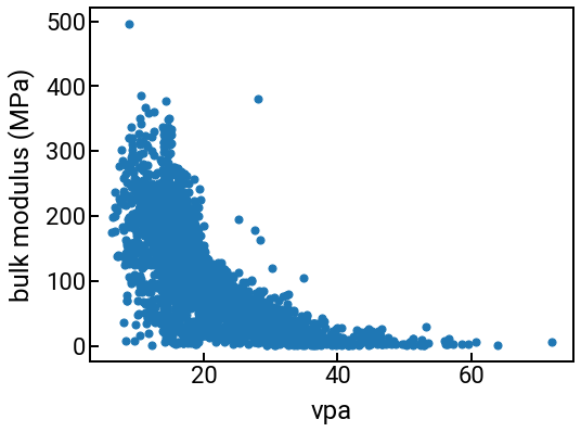
What can we do with these new features?

Same thing as before! Since we like plots, let’s make a few plots. 🙂

Scatter plot

single_feature = struct_feature_labels[1]   # we pick one that's kinda cool
fig, ax = plt.subplots()
ax.scatter(df_struct[single_feature], df_struct['bulk_modulus'], s=50)
ax.set_xlabel(single_feature)
ax.set_ylabel('bulk modulus (MPa)')
plt.show()

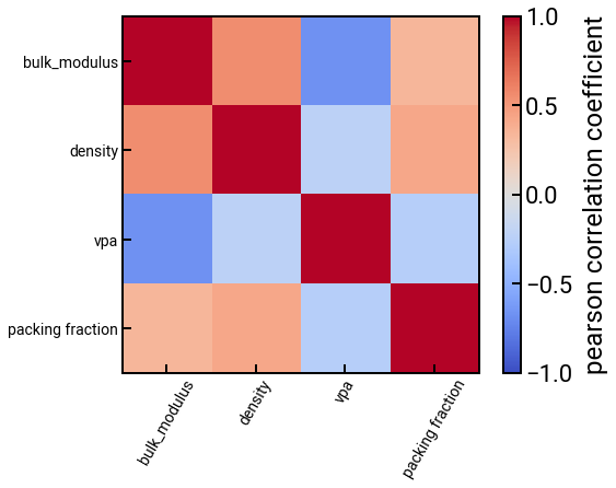
Correlation matrix

# trim the DataFrame
features_subset = ['bulk_modulus'] + struct_feature_labels
df_subset = df_struct[features_subset]

# construct a correlation matrix
method = 'pearson'
corr_matrix = df_subset.corr(method=method)

# plot the correlations
fig, ax = plt.subplots()
h = ax.imshow(corr_matrix, cmap='coolwarm', vmin=-1, vmax=1)
ax.set_xticks(range(len(features_subset)))
ax.set_xticklabels(features_subset, rotation=60, fontsize=14)
ax.set_yticks(range(len(features_subset)))
ax.set_yticklabels(features_subset, fontsize=14)
plt.colorbar(h, label=f'{method} correlation coefficient')
plt.show()

Conclusion

Back to top

This concludes the review of matminer. If you have any questions, please do not hesitate to ask on Slack!

Proposals Day 09: Research