.ipynb .pdf

repository open issue suggest edit

JupyterHub Colab

Contents

Introduction to ML notebook

Authors: Enze Chen and Mark Asta (University of California, Berkeley)

Note

This is an interactive exercise, so you will want to click the and open the notebook in DataHub (or Colab for non-UCB students).

Learning objectives

This notebook contains a series of exercises that will teach you the basics of machine learning (ML) and the scikit-learn package, which is a very popular framework for ML in Python. We will start with a discussion of common terms and conventions in ML so that everyone is on the same page, and then cover our first supervised learning algorithm: linear regression. By the end of this lesson, you will be able to:

1. Define the common terminology used in ML.

2. Write a vanilla gradient descent algorithm for linear regression.

3. Use scikit-learn to construct linear regression models.

We will progress through most of this exercise together as a group and are happy to take questions you might have.

Contents

These exercises are grouped into the following sections:

1. Overview of ML

2. Regression by hand

3. Regression with scikit-learn

4. Classification (bonus)

Overview of ML

Back to top

We will start by covering some fundamental ideas and terminology in ML. These were all discussed in the live Zoom session, so we will only provide a quick summary here.

The three broad types of ML problems/applications are

1. Regression for predicting a numerical value.

2. Classification for predicting a categorical value.

3. Clustering for identifying structure in data.

A roughly parallel classification in terms of learning algorithms is

1. Supervised learning, where inputs and outputs are given. Regression and classification mostly correspond to supervised learning.

2. Unsupervised learning, where inputs are given but outputs are not. Clustering mostly corresponds to unsupervised learning.

Regression by hand

Back to top

We will start with supervised learning algorithms for regression, where the input data in design matrix $X\in {\mathbb{R}}^{m\times n}$ and output target vector $\overrightarrow{y}\in {\mathbb{R}}^m$ are both provided.

Each row of $X$ and $\overrightarrow{y}$ is a corresponding example or data point (so there are $m$ examples), and each column of $X$ is a feature (so there are $n$ features).

Our job is to learn a function/model $h(X,\overrightarrow{\theta })$ that tries to map $X\to \overrightarrow{y}$ using a set of parameters $\overrightarrow{\theta }\in {\mathbb{R}}^n$. So far this is a general formulation.

The model $h(X,\overrightarrow{\theta })$ can vary in complexity, and generally we classify the function/model as linear or nonlinear, where linear here specifically refers to “a function that is linear in the parameters $\overrightarrow{\theta }$.” This means the function will have linear terms ${\theta }_1$, ${\theta }_2$, etc., but no cross-terms like ${\theta }_1{\theta }_2$. We can imagine one such linear model could be:

$$h(X,\overrightarrow{\theta })=X\overrightarrow{\theta }={\theta }_1{\overrightarrow{x}}_1+\cdots +{\theta }_n{\overrightarrow{x}}_n=\hat{y}$$

which is the vectorized form of multivariable linear regression. Our goal is to find a set of parameters $\overrightarrow{\theta }$ such that $X\overrightarrow{\theta }=\hat{y}$ closely approximates $\overrightarrow{y}$. Recall that $X$ and $\overrightarrow{y}$ are the data (known), while $\overrightarrow{\theta }$ is what we’re trying to figure out (unknown). $\hat{y}$ are the model’s predictions and the process of learning the parameters $\overrightarrow{\theta }$ is called training the model.

---

Pause and reflect: Why might we start with a linear model?

Cost function

How can we measure if we’re close? For a single example ${\overrightarrow{x}}^{(i)\mathrm{\top }}\in {\mathbb{R}}^n$ in row $i$ of $X$, we can compute the squared error:

$$({\hat{y}}^{(i)}-y^{(i)}{)}^2=({\overrightarrow{x}}^{(i)\mathrm{\top }}\overrightarrow{\theta }-y^{(i)}{)}^2$$

If we want to find the total error across all examples, we then add across all rows $i$:

$$\begin{array}{}\text{(1)}& \sum _{i=1}^m({\overrightarrow{x}}^{(i)\mathrm{\top }}\overrightarrow{\theta }-y^{(i)}{)}^2\end{array}$$

If we think a little bit about this expression and try to express the same idea in matrix-vector notation, we can rewrite Eq 1 as:

$$||X\overrightarrow{\theta }-\overrightarrow{y}|{|}_2^2=||\hat{y}-\overrightarrow{y}|{|}_2^2$$

Another word to describe this quantity is the cost function, symbolized $J$, which measures the “price we pay” (penalty) for this approximate linear model. It is customary to include a factor of $\frac{1}{2}$ in the cost function for reasons you’ll see shortly, and normalize the cost function by the number of examples $m$. Thus, the cost function for our linear regression model is:

$$\begin{array}{}\text{(2)}& J(\overrightarrow{\theta })=\frac{1}{2m}||X\overrightarrow{\theta }-\overrightarrow{y}|{|}_2^2\end{array}$$

---

Pause and reflect: Why is $J$ a function of $\overrightarrow{\theta }$?

Learning through optimization

Now that we have an expression for the penalty (Eq 2), we have a path forward towards learning the “best model” by trying to minimize this function. And we know that to minimize functions, we have to take a derivative, which in higher dimensions you’ll know as the gradient, and set the result equal to $0$.

In multivariable calculus, you took the gradient of a scalar potential (like gravitation, electric, or arbitrary), but here we’re taking the gradient of a vector norm and applying chain rule to a matrix-vector product. While the details are unfortunately outside the scope of this lesson, the result is:

$$\begin{array}{}\text{(3)}& {\mathrm{\nabla }}_{\theta }J(\overrightarrow{\theta })=\frac{1}{m}{X}^{\mathrm{\top }}(X\overrightarrow{\theta }-\overrightarrow{y})\end{array}$$

where the power rule cancels out the $\frac{1}{2}$ and we apply the multidimensional chain rule to get the $X^{\mathrm{\top }}$ out front. We can then solve for the optimal parameters $\overrightarrow{\theta }$ in two ways.

The first, as alluded to above, is to set the gradient equal to $\overrightarrow{0}$ since that will be the location of the minimum. Doing this and rearranging terms, we get the normal equation solution to least-squares linear regression:

$$\begin{array}{}\text{(4)}& \overrightarrow{\theta }=(X^{\mathrm{\top }}X{)}^{-1}{X}^{\mathrm{\top }}\overrightarrow{y}\end{array}$$

Exercise: linear regression

We will return to the problem from the first day of predicting the atomic weight of an element from the atomic number. Recall that the physical relationship is:

$$\text{atomic weight = atomic number + weighted-average number of neutrons}$$

Import Python packages

import numpy as np
import pandas as pd
import matplotlib.pyplot as plt
%matplotlib inline

plt.rcParams.update({'figure.figsize':(8,6),       # Increase figure size
                     'font.size':20,               # Increase font size
                     'mathtext.fontset':'cm',      # Change math font to Computer Modern
                     'mathtext.rm':'serif',        # Documentation recommended follow-up
                     'lines.linewidth':5,          # Thicker plot lines
                     'lines.markersize':12,        # Larger plot points
                     'axes.linewidth':2,           # Thicker axes lines (but not too thick)
                     'xtick.major.size':8,         # Make the x-ticks longer (our plot is larger!)
                     'xtick.major.width':2,        # Make the x-ticks wider
                     'ytick.major.size':8,         # Ditto for y-ticks
                     'ytick.major.width':2,        # Ditto for y-ticks
                     'xtick.direction':'in', 
                     'ytick.direction':'in'})

Normal equations - as a team!

We’ll import the data from the number_weight.npy file, which is structured as

$$\begin{array}{r}\text{data}=\left[\begin{array}{cc}1& 1.008\\ 2& 4.003\\ ⋮& ⋮\\ 49& 114.818\\ 50& 118.71\end{array}\right]\end{array}$$

and what we want is

$$\begin{array}{r}X\equiv \left[\begin{array}{cc}\overrightarrow{1}& \overrightarrow{Z}\end{array}\right]=\left[\begin{array}{cc}1& 1\\ 1& 2\\ ⋮& ⋮\\ 1& 49\\ 1& 50\end{array}\right],\overrightarrow{y}=\left[\begin{array}{c}1.008\\ 4.003\\ ⋮\\ 114.818\\ 118.71\end{array}\right]\end{array}$$

which allows us to get $\overrightarrow{\theta }$ through

$$\begin{array}{}\text{(4)}& \overrightarrow{\theta }=(X^{\mathrm{\top }}X{)}^{-1}{X}^{\mathrm{\top }}\overrightarrow{y}\end{array}$$

Hints:

• np.column_stack() arranges 1D arrays vertically into a 2D array.

• np.reshape(arr, (-1, 1)) can take a 1D array and force it into a column vector.

• @ is the matrix multiplication operator, and X.T is the transpose of array X.

• np.linalg.inv(arr) computes the inverse of a 2D array.

• We can plot the result now with our matplotlib prowess. Let’s see what atomic weights our model predicts for the original atomic numbers stored inside X.

data = np.load('../../assets/data/week_1/01/number_weight.npy')
# -------------   WRITE YOUR CODE IN THE SPACE BELOW   ---------- #

# --------------------------------------------------------------- #
fig, ax = plt.subplots()
ax.scatter(X[:, 1], y, label='data')
ax.plot(X[:, 1], X @ theta, 'gray', label='regression')
ax.set_xlabel('atomic number')
ax.set_ylabel('atomic weight')
ax.legend()
plt.show()

Gradient descent - as a team?

The second method for solving linear regression is through gradient descent, which is an iterative approach. In parameter space, we are searching for the minimum of $J(\overrightarrow{\theta })$ which is a convex function. This means we can make an initial guess for $\overrightarrow{\theta }$ and slowly move in the direction opposite the gradient at that point to get ourselves closer to the minimum. This is the idea behind gradient descent and the update rule looks like:

$$\begin{array}{}\text{(5)}& {\overrightarrow{\theta }}_{\text{new}}:={\overrightarrow{\theta }}_{\text{old}}-\alpha {\mathrm{\nabla }}_{\theta }J(\overrightarrow{{\theta }_{\text{old}}})\end{array}$$

where $\alpha$ is a step size or learning rate. By repeating this update rule again and again (and again and again and again…), we can arrive at our solution.

Exercise: implement gradient descent for linear regression

Recall that the cost function is given by:

$$\begin{array}{}\text{(2)}& J(\overrightarrow{\theta })=\frac{1}{2m}||X\overrightarrow{\theta }-\overrightarrow{y}|{|}_2^2\end{array}$$

and its gradient wrt $\overrightarrow{\theta }$ is

$$\begin{array}{}\text{(3)}& {\mathrm{\nabla }}_{\theta }J(\overrightarrow{\theta })=\frac{1}{m}{X}^{\mathrm{\top }}(X\overrightarrow{\theta }-\overrightarrow{y})\end{array}$$

The gradient descent update rule is given as

Loop until we decide to stop: $$\begin{array}{}\text{(5)}& \overrightarrow{\theta }& =\overrightarrow{\theta }-\alpha {\mathrm{\nabla }}_{\theta }J(\overrightarrow{\theta })\end{array}$$

Hints:

• Write should write a separate helper function, but we only need one. Which one?

• Initialize $\overrightarrow{\theta }=\left[\begin{array}{c}0\\ 0\end{array}\right]$ and $\alpha ={10}^{-3}$.

• How do we know when to stop?

X = np.column_stack([np.ones(m), data[:, 0]])
y = np.reshape(data[:, 1], (-1, 1))   # need to force 2 dimensions for this exercise
# -------------   WRITE YOUR CODE IN THE SPACE BELOW   ---------- #

# --------------------------------------------------------------- #
print(f'The parameters are {theta.ravel()}.')
print(f'It took {iters} iterations to optimize.')

fig, ax = plt.subplots()
ax.scatter(X[:, 1], y, label='data')
ax.plot(X[:, 1], X @ theta, 'gray', label='regression')
ax.set_xlabel('atomic number')
ax.set_ylabel('atomic weight')
ax.legend()
plt.show()

Pause and reflect: How do the results from gradient descent compare to those from the normal equations?

Animated version

To showcase another cool matplotlib module, matplotlib.animation, we will animate the process of gradient descent using the following code so you can visualize the algorithm learning the parameters with each step. Seeing is believing, as they say. 👀

You should be able to directly run the following code. Note that we’re stopping it early so it’s not yet fully optimized, but the remaining iterations aren’t too interesting.

from matplotlib.animation import FuncAnimation
from matplotlib.artist import Artist
data = np.load('../../assets/data/week_1/01/number_weight.npy')
m = len(data)
X = np.column_stack([np.ones(m), data[:, 0]])
y = np.reshape(data[:, 1], (-1, 1))
theta = np.zeros((2, 1))
ALPHA = 1.8e-3
cost = 1 / (2 * m) * np.linalg.norm(X @ theta - y) ** 2

fig, ax = plt.subplots()
ax.scatter(data[:, 0], data[:, 1], label='data')
h, = ax.plot([], [], c='gray', label='regression')
ax.set_xlabel('atomic number')
ax.set_ylabel('atomic weight')
FONTSIZE = 18
ax.legend(loc=(0.55, 0.2), fontsize=FONTSIZE)
t = ax.text(0, 0, '')
u = ax.text(0, 0, '')
v = ax.text(0, 0, '')
plt.tight_layout()
plt.close()

def init():
    return h,
    
def animate(i):
    global cost, theta, X, y, ax, t, u, v
    h.set_data(data[:, 0], X @ theta)
    Artist.remove(t)
    Artist.remove(u)
    Artist.remove(v)
    box = dict(fc='1.0', ec='white')
    t = ax.text(2, 110, s=f'iteration {i}', fontsize=FONTSIZE, ha='left', bbox=box)
    u = ax.text(2, 95, s=f'cost = {cost:.3f}', fontsize=FONTSIZE, ha='left', bbox=box)
    v = ax.text(2, 80, s=rf"$\theta$ = {theta.ravel()}", fontsize=FONTSIZE, ha='left', bbox=box)
    
    theta = theta - ALPHA * (X.T @ (X @ theta - y)) / m
    cost = 1 / (2 * m) * np.linalg.norm(X @ theta - y) ** 2
    return h, t, u, v

plt.rcParams.update({'animation.html': 'jshtml'})
np.set_printoptions(precision=3)
anim = FuncAnimation(fig, animate, init_func=init, frames=30, interval=400, repeat=False);
anim

Once Loop Reflect

~ BREAK ~ At this point, we're going to give ourselves a short break before continuing further. Great work so far! 💪

Regression with scikit-learn

Back to top

Now that you’ve cleared the rite of passage in ML, it’s time to introduce a package that will simplify our lives. 🙏 Scikit-learn is one of the most popular packages for ML in Python, and it’s designed in a modular way to be extremely user-friendly. It has all sorts of ML algorithms implemented for us and has great documentation with examples. Perhaps one of the annoying downsides is that the package is so modular that some of the sub-modules can be pretty hard to find sometimes, but luckily you are all expert documentation searchers. 🕵️‍♀️🕵️‍

To use scikit-learn, the typical import statement is:

from sklearn.module import ClassWeWant

where you’ll note that the root package name is sklearn!

Step 1: As an example, to perform linear regression, we import the LinearRegression class from the linear_model module as follows:

from sklearn.linear_model import LinearRegression

Step 2: We then create an object from this class (e.g., lr = LinearRegression()).

Step 3: We can train the model on a design matrix $X$ and target vector $y$ using the lr.fit(X, y) method, which operates in place. Note that if $X$ has a column of $\overrightarrow{1}$, then we will also want to pass fit_intercept=False into this method. If our design matrix does not have an intercept term explicitly encoded, then we can leave it as the default (True for fit intercept term separately).

Step 4: A trained model has coefficients that are accessible through the lr.coef_ attribute (ndarray type). This is our $\overrightarrow{\theta }$, which the package automatically optimized (trained) for you. If the intercept term was fit separately (not in design matrix), then that is accessed through the intercept_ attribute (likely a float in our case). We can use these coefficients to create the equation for a line of best fit, which we’ll do here.

We can also use a trained model to make predictions on new data $X^{\prime }\in {\mathbb{R}}^{p\times n}$ by calling lr.predict(Xp), which returns a vector of predictions $\hat{y}$. In some cases, we’d like to plot the predicted values—more on this shortly!

Exercise: use scikit-learn to train a linear regression model for the atomic weights problem and plot the line of best fit

Hint:

• We’ve loaded the training data for you, and the process to fit the data should take only 4 lines of code(!!)

• Once you’ve fit the model, we suggest you print out the coefficients and intercept terms. Do they match the results from above? 😀

data = np.load('../../assets/data/week_1/01/number_weight.npy')
X = np.reshape(data[:, 0], (-1, 1))   # NO INTERCEPT TERM (no extra column of 1s)
y = data[:, 1]
# -------------   WRITE YOUR CODE IN THE SPACE BELOW   ---------- #

fig, ax = plt.subplots()
ax.scatter(X, y, label='data')
ax.plot(X, lr.coef_[0] * X_scaled + lr.intercept_, 'gray', label='regression')
ax.set_xlabel('atomic number')
ax.set_ylabel('atomic weight')
ax.legend()
plt.show()

Pause and reflect: Based on what you’ve seen so far with scikit-learn, and comparing this work to our previous exercises on data management and data visualization, what does this suggest (at least preliminarily) about the “distribution of effort” in MI pipelines?

Classification (on your own)

Back to top

Now let’s try our hand at a classification problem, where our goal is to build a model that can learn the correct labels for our data, such as {metal, non-metal}. These labels are also stored in our target vector $\overrightarrow{y}$, except now the values in $\overrightarrow{y}$ can only take on a few discrete values instead of any real number. To simplify the problem even further, we will consider the problem of binary classification, where there are only two classes (labels) for us to consider. One way to programmatically represent these classes is with the values $\{0,1\}$, which conveniently makes the logistic function a good model for classifying this data.

fig, ax = plt.subplots()
x = np.linspace(-6, 6, 100)
y = 1 / (1 + np.exp(-x))
b = np.zeros(len(x))
t = np.ones(len(x))
ax.plot(x, b, 'gray', ls='dashed')
ax.plot(x, t, 'gray', ls='dashed')
ax.plot(x, y)
ax.text(-5, 0.7, s=r'$g(z) = \dfrac{1}{1 + e^{-z}}$')
ax.set_xlabel('$z$')
ax.set_ylabel('$g(z)$', rotation=0, labelpad=35)
plt.show()

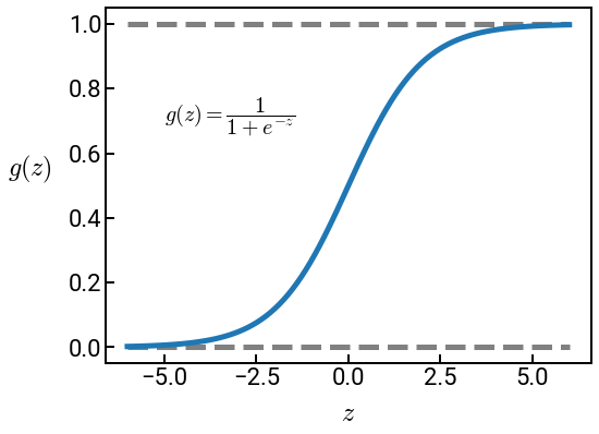
As can be seen from the plot, the logistic function is bounded between $g(z)\in (0,1)$. For very large (positive) values of $z$, the function approaches $1$, while for very small (negative) values of $z$, the function approaches $0$. When the argument $z=0$, the value of the function is $g(z)=0.5$.

This means we could use the output of this function as a classifier based on the input argument. When the logistic function has the particular input:

$$h(X,\overrightarrow{\theta })=g(X\overrightarrow{\theta })={\displaystyle \frac{1}{1+\exp (-X\overrightarrow{\theta })}}$$

we call this model logistic regression. It has a nice probabilistic interpretation, where $h(X,\overrightarrow{\theta })$ is the probability of the data point being class 1 and $1-h(X,\overrightarrow{\theta })$ the probability of the data point being class 0.

Note that there is “regression” in the name of this method, but it’s fundamentally for classification! Like linear regression, logistic regression is also a linear algorithm (still only a dot product). Although we will not show it, logistic regression even has the same gradient descent update rule for learning $\overrightarrow{\theta }$!

Exercise: use scikit-learn to classify elements by metal, non-metal

Hints:

• The data has been loaded for you in a pandas DataFrame, and the target output is in the is_metal column.

• The arrays $X$ and $\overrightarrow{y}$ are structured the same way as for linear regression, and you can pick your input features! We suggest row and group to start with.

• Recall that we select multiple columns using df[list_of_column_names], even for a single column. By this we mean:

X = df[['atomic_number', 'row']]   # this is good; a list of 2 column names
X = df[['atomic_number']]          # this is good; a list of 1 column name
X = df['atomic_number']            # avoid this!!! a string of 1 column name

• After training your model, evaluate it on the original training data, but call lr.predict_proba(X), which returns probability estimates for each class, and not just the binary class.

• Please store your predictions in the yhat variable and uncomment the rest of the code.

df = pd.read_csv('../../assets/data/week_1/04/elem_props.csv')
df.head()
X = df[['row', 'group']]   # try changing these up!
y = df['is_metal']
X_scaled = scaler.fit_transform(X)
# -------------   WRITE YOUR CODE IN THE SPACE BELOW   ---------- #

# --------------------------------------------------------------- #
from pymatgen.util.plotting import periodic_table_heatmap    # more pymatgen fun
plot_data = {}
for i in range(len(yhat)):
    plot_data[df['symbol'][i]] = yhat[i][1]   # get the second class probabilities
ptable = periodic_table_heatmap(elemental_data=plot_data, cmap='coolwarm')

Conclusion

This concludes the introduction to ML, which admittedly was a lot! We discussed regression and classification problems, which are both solved with supervised learning algorithms. We coded up linear regression with gradient descent by hand to get a feel for the algorithms, but then quickly turned to the scikit-learn package, which we’ll continue to rely on for the rest of this module.

We’d love to take any questions you may have, and if you need some time to let the information sink in (and questions to form), that’s understandable. Next up we’re going to discuss various ways of measuring model performance to better quantify what makes a “good” ML model.

Introduction to ML Quantifying performance