Introduction to Python and Jupyter notebooks
Authors: Enze Chen and Mark Asta (University of California, Berkeley)
Welcome! In this notebook, we will introduce the Python programming language and Jupyter notebook programming environment. If you already have extensive experience with both of these concepts, that’s great! We hope you don’t mind the quick refresher, and maybe some of our protips will be new for you. 😀
Note
This is an interactive exercise, so you will want to click the and open the notebook in DataHub (or Colab for non-UCB students).
Did you say… Python?
Fig. 1 Python logo.
By now, many people know (or at least have heard of) the Python programming language, but what they don’t know is that the language is not named after the snake 🐍, but rather the television show Monty Python’s Flying Circus! 📺
Since its introduction in 1991, Python has skyrocketed in popularity in recent years to become one of the most popular programming languages used in computer science, and arguably the most popular language in data science. This growth is in part due to:
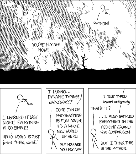
Fig. 2 xkcd comic 353.
Its readability. Python is designed to be simple and reads like English, using common keywords instead of symbols (e.g.,
andvs.&&).Its extensibility. Python makes it easy for developers to write modules that extend its functionalities for applications in data science, scientific computing, imaging black holes, and flying drones on Mars.
Its open-source properties. This means anyone can contribute to Python development and anyone can use it—for free!
For these reasons (and more), we will be using Python for this module. If you’re new to Python, that’s OK! The rest of today will be spent on [re]acquainting ourselves with Python and introducing the necessarity functionalities.
Using Python code
In this module, we’re going to take a somewhat practical approach to using Python, in the sense that we view it as just another tool in our toolbox for expanding our understanding of materials. We’ll discuss Python concepts, syntax, and style along the way, but the focus will always be on applying it to solve relevant MSE problems in a data-driven fashion. Therefore, our focus as mentors will be to teach you only what’s relevant for this module, and unfortunately won’t have much time to extensively cover the details of the language or various packages during the tutorials (you’re welcome to ask in OH!).
While this strategy risks leaving you with only a cursory understanding of Python, we want to offer three points of solace and why this might not actually be the case:
Based on the initial survey, many of you have some programming experience already, even if it’s in a different language. We think you’ll be surprised to find that, both at a theoretical and applied level, Python is not too different from other languages that you may have seen (e.g., C++, MATLAB) and that a lot of your prior knowledge will transfer to help you understand Python.
Solving scientific problems algorithmically (e.g., in a data-driven way) often requires a lot more than being able to program, irrespective of the programming language. Therefore, while we’re teaching you Python programming syntax and tools, what we’re really hoping to communicate is a way of thinking like a computer, which is quite different than the way humans think. And so you might find that you’re spending more time formulating data-driven solutions than actually writing code. A little planning goes a long way. For more on this topic, see Jeannette Wing’s article on computational thinking assigned in the Homework.
The third point isn’t really related to Python but to the internship more broadly, and that is our desire to expose you to the graduate school research experience, which encompasses a lot more than hammering out lines of code. We have designed this module in such a way that surfaces these other elements (the pleasant ones, anyways 😉) which we hope you will come to appreciate as well.
Running Python code
You can write Python code just about anywhere (even in Microsoft Word, lol), but in order to execute the code, you will need a Python kernel. For this module (at least, for these tutorials), we will use Jupyter notebooks for running the Python code we write.
Philosophy of Jupyter notebooks
The main design philosophy behind Jupyter notebooks could be summarized as the following: A platform for creating computational narratives to promote literate computing. The creators of Project Jupyter, one of whom is UC Berkeley Statistics Professor Fernando Pérez, wanted to create a tool that made computational research easier to communicate and more reproducible, which led to the development of Jupyter notebooks. The interleaving of code with prose and graphics has made programming a lot more accessible to general audiences and the interactivity of these notebooks also makes them great teaching tools!
Organization of Jupyter notebooks
The information in Jupyter notebooks is organized into cells, which come in many forms.
This cell is called a Markdown cell, which is used for text that can be formatted with the Markdown markup language.
This is a fairly simple, yet extremely powerful markup language that allows you to do most of the basic styles, such as add emphasis, make itemized lists, create headings, write inline code, add links, include external images, and use HTML (see here for a cheat sheet).
You know this is a Markdown cell because when you select this cell (click on it such that a blue bar appears on the left), the menu bar at the top shows “Markdown v” in the second row:

As an example, here is an itemized list:
spam
eggs
And here is a code block in the Markdown cell with Python syntax highlighting:
print('Hello, World!')
And if you love \(\LaTeX\) as much as we do, it can handle that too. 😍
Making edits
To edit a Markdown cell, double-click on it until you see your cursor flashing in the cell and the cell change color from blue to green. The cell’s background will also change color from white to a light gray.
EXERCISE: Double click on this cell and answer the following question by replacing the underscores:
What is your name? _________
To leave “edit mode” and show your changes, press Shift+Enter when you’re done.
Notice how we included several Markdown cells in a row rather than putting all this information into a single, giant cell. It’s often a nice design choice to split your work into smaller chunks to improve readability. 👀
Introducing the code cell
Notice how the next cell looks a little different. It is a code cell, which you can distinguish in a few ways.
If you click in the cell, the menu bar at the top will now show “
Code v.”The cell will always have a gray background.
You may also notice a
In [ ]:tag in the left margin.
You can write Python code in these cells and then execute the code with Shift+Enter. Or you can click the ▶ Run button in the menu bar.
EXERCISE: In the space below, enter your name between the quotation marks and then run the code cell.
# inline comments in Python start with "#"
name = ""                  # enter your name here as a string
print(f'Hello, {name}!')   # this is a formatted string literal, or f-string, and it's f-ing awesome
Now you might notice that some output appeared after you executed the cell (which makes sense because we called print()) and a number also appeared between the square brackets!
(e.g., In [1]:)
This number indicates the sequence of code cell execution, which can be handy for a few reasons:
You can clearly tell which cells have been executed and which cells have not. A cell’s variables and functions are only usable in the notebook after it has been executed.
Accordingly, for better or worse, the variables and functions in one code cell (at the global scope) can be accessed in other code cells that are executed later. This allows you to split code among several code blocks and run them sequentially.
For better or worse, you can execute code cells in Jupyter notebooks in whatever order you want. We still recommend top to bottom, but this does give us flexibility to change an earlier code cell (and rerun it!) if we later deem it necessary.
DataHub
If you are a UC Berkeley student, you may be reading this Jupyter notebook on the school’s DataHub (a JupyterHub instance), which has been graciously provisioned for this module by the Division of Computing, Data Science, and Society. With DataHub, all of our Python code will be saved and executed in the cloud, which saves us a lot of hassle with software installation. Everything is also automatically synced with the Jupyter Book!
Installing extra packages
Perhaps the only “catch,” which may come up as you work on your research project, is that you will still have to manually install Python packages that are not included with the default DataHub deployment every time you load DataHub.
In order to install new packages, use the pip package manager directly within a Jupyter code cell.
EXERCISE: Let’s demonstrate this below by adding a new code cell and installing the mendeleev package.
We’ll also quickly demonstrate how to navigate to the root directory for you to see all the files in DataHub and upload new ones as needed. Note that when you close a DataHub notebook, your edits and outputs are preserved, but the variables (kernel) will be reset.
General programming principles and tips ☝
EXERCISE: Before we set you loose to work on practice problems, let’s spend some time discussing some general programming principles and best practices.
I’ll start us off with one: save your work frequently. Just because a code cell runs or a Markdown cell renders does not mean that your work is saved. Jupyter notebook kernels are known to crash pretty randomly, so save your work by clicking the symbol in the menu bar or using Ctrl+S (or Command+S on Macs).
Resources
If you want to read more about the design of Jupyter notebooks, please see the short paper by Kluyver, T. et al. Positioning and power in academic publishing: Players, agents and agendas, 2016.
If you want to see a [very long] list of interesting Jupyter notebooks, see here.
More tutorials on using Python in Jupyter notebooks can be found with a quick web search.
For a Markdown cheat sheet, see here.