Python: The greatest hits
Authors: Enze Chen and Mark Asta (University of California, Berkeley)
Note
This is an interactive exercise, so you will want to click the and open the notebook in DataHub (or Colab for non-UCB students).
This notebook contains a series of exercises that are intended for people who already have some Python experience. If you’re able to complete the exercises without too much difficulty (note: use of Google and Stack Overflow is not only allowed, but encouraged), then you’re in good shape for the rest of this module. There are many, many Python tutorials out there, so we’ve tried to make these exercises as relevant to MSE as possible. If there is a concept that is new to you, feel free to hop over to the “Python: The gory details” notebook for more information, or just ask us.
Contents
These exercises are grouped into the following sections:
Strings and lists
Exercise: string vs. list
First a conceptual question: Identify one way string and list are similar in Python and one way they’re different.
Write your answer here by editing this Markdown cell.
Answer: ____
Exercise: parsing strings
Often times when working with data, files, etc., we have to take slices of strings (substrings), split them, join them, etc. This can be to extract the name of a compound, a date, an experimental parameter, etc. Since we have a lot of data, we would like to come up with a robust algorithm that can flexibly handle a variety of inputs (assuming that some overall structure is maintained—not always a safe assumption in the wild!).
Your colleague gives you a list of files with absorption data and asks you to extract the chemical formulas from the file path and store them into a list.
They would also like to have the collection date stored in the format MM-DD-YY with hyphens instead of the default underscores generated by the program.
The data input list of files is provided below, and your job is to create two lists that look like:
formulas = ['Si', 'GaAs', 'InP', 'AlGaAs']
dates = ['06-28-21', '06-28-21', '06-29-21', '06-30-21']
Hints:
You might want to apply
forloops,str.split(),str.join(), and indexing/slicing.We recommend thinking through all the steps required to solve this problem before jumping into the code. Write some comments (or pseudocode) to help guide your computational thinking process.
We also recommend solving this problem iteratively, doing one string operation at a time and verifying that step works.
data = ['path/to/absorption/data/Si_06_28_21.txt',
        'path/to/absorption/data/GaAs_06_28_21.txt',
        'different/path/to/absorption/data/InP_06_29_21.txt',
        'path/to/more/absorption/data/AlGaAs_06_30_21.txt']
# -------------   WRITE YOUR CODE IN THE SPACE BELOW   ---------- #
Exercise: functions and lists

Now we’ll go through another exercise with lists, this time by writing your own helper function.
Mark gives you some data on band gaps, but his evil twin Kram changed the values from float to string.
This makes it difficult to work with (try running the code below).
Write a helper function that takes the list of string as input and returns a list of corresponding floats. Also return the minimum and maximum values in the list. Finally, call the function on the band gap data to ensure it works as expected. Your final returned result should be similar to:
([1.14, 1.43, 0.67, 5.5, 3.4, 0.37, 0.0001, 10.0], 0.0001, 10.0)
band_gaps = ['1.14', '1.43', '0.67', '5.5', '3.4', '0.37', '1e-4', '1e1']
print(f'The maximum band gap value in the original list is {max(band_gaps)} eV')   # ???
# -------------   WRITE YOUR CODE IN THE SPACE BELOW   ---------- #
The maximum band gap value in the original list is 5.5 eV
Working with files
Most of the time, our data will be stored in external files rather than hard coded like the previous examples, so we have to be proficient in working with files. On Tuesday, we’ll be going through several examples with different file formats that are commonly used in MI, but for now we’ll practice reading in a text file with data containing the ground-state crystal structure of the elements.
Materials structure
First, we’ll discuss a little bit about the science to provide context and motivation. In MSE, we are often concerned with the characteristics of and relationships between four central tenets: processing, structure, properties, and performance (PSPP). As all of these points heavily influence each other, their relationship (and thus, the whole endeavor of MSE) is typically summarized by the following schematic from Wikipedia:

In this exercise, we’re focusing on the structure component of the above tetrahedron. But note that when we talk about “materials structure,” there are actually many possible length scales on which we can describe the structure.
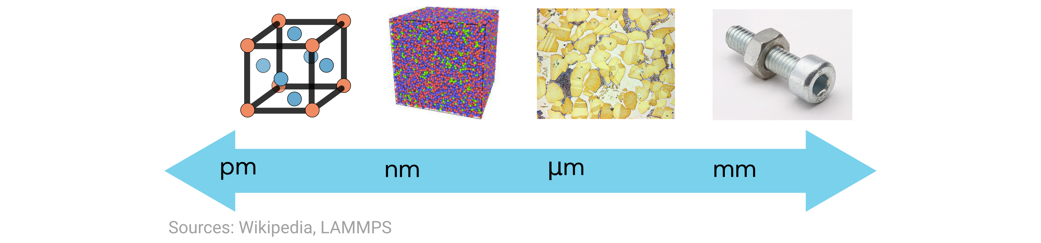
In this problem, we’re looking at the ground-state crystal structure of the elements, which is on the far-left end of the above scale. Here the length scales are typically on the order of Angstroms, or \(10^{-10}\) meters. Moreover, the crystal structures of all crystalline materials can be classified into 14 different Bravais lattices that can be further grouped into six crystal families, as shown here:
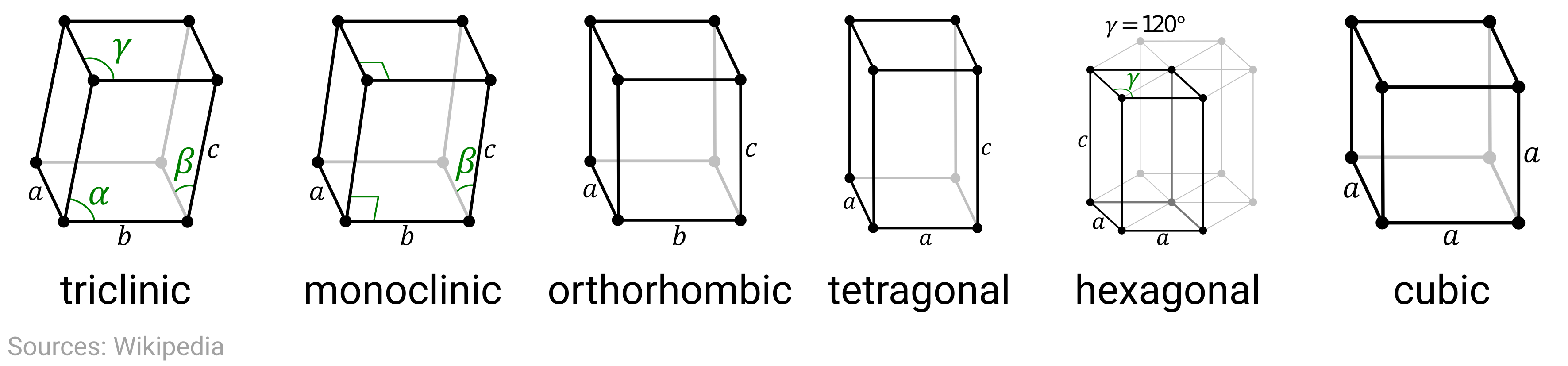
The crystal structure (lattice + basis) determines the symmetries of the system and has considerable influence on the physical, mechanical, optoelectronic, and magnetic properties of the material. Later this week, we’ll see how we can encode and leverage this structural information to aid our data analysis.
Exercise: Reading files
We’ve included a file element_structure.txt that contains information on the crystal family of the first 50 elements in the periodic table.
The first few lines of the file look like:
# Data from https://periodictable.com/Properties/A/CrystalStructure.html
Hydrogen Hexagonal
Helium Cubic
Lithium Cubic
Beryllium Hexagonal
where there’s a comment in the first line and the subsequent lines are the element and family separated by a single space. In this first example, read in the file and print out the first ten elements along with their atomic number. You should not have to rely on other packages, just native Python. Your output should look something like this (leading zeros are bonus points!):
01 Hydrogen
02 Helium
...
10 Neon
Hint: You might want to use enumerate(), continue, break, str.startswith(), and str.split().
crystal_data = '../../assets/data/week_1/01/element_structure.txt'
# -------------   WRITE YOUR CODE IN THE SPACE BELOW   ---------- #
Exercise: creating a dictionary
Using the same file as the previous exercise, read in the data from the file and store them into a dictionary where the key:value pairs are element:family.
The first few entries of the dictionary will look similar to (order might be different; that’s OK):
{'Hydrogen': 'Hexagonal',
 'Helium': 'Cubic',
 'Lithium': 'Cubic',
 'Beryllium': 'Hexagonal',
 ...
Dictionaries are nice because they serve as quick lookup tables when we want to find associated values. For those who have learned a bit about algorithmic efficiency, you might be interested to know that a Python dictionary has constant lookup time, whether that dictionary has ten or ten million entries!
crystal_data = '../../assets/data/week_1/01/element_structure.txt'
# -------------   WRITE YOUR CODE IN THE SPACE BELOW   ---------- #
Exercise: inverting the dictionary
Now take that dictionary you created in the previous exercise and “invert” it. By this, we mean turn the values into keys and keys into values (still corresponding). Doing this allows us to, for example, find all elements that have a similar crystal structure, if we’re only searching for materials with that structure.
Notice that because keys have to be unique in a dictionary, the same crystal family (e.g., Cubic) will correspond to multiple elements (e.g., Helium, Lithium, Neon).
Therefore, the value corresponding to each key in the inverted dictionary should be a list of all the elements belonging to that family.
Your code takes the previous dictionary as input and returns another dictionary that will look similar to (order of keys and values doesn’t matter):
{'Hexagonal': ['Hydrogen', 'Beryllium', 'Carbon', ...],
 'Cubic': ['Helium', 'Lithium', 'Neon', ...],
 'Trigonal': ['Boron', 'Arsenic'],
 'Monoclinic': ['Oxygen', 'Fluorine', 'Selenium'],
 'Triclinic': ['Phosphorus'],
 'Orthorhombic': ['Sulfur', 'Chlorine', 'Gallium', 'Bromine'],
 'Tetragonal': ['Indium', 'Tin']
}
Hint: You might have to check to see if a value from the original dictionary (i.e. crystal family) current exists as a key in your new dictionary.
# ------------- WRITE YOUR CODE IN THE SPACE BELOW ---------- #
Working with NumPy
In this last section, we’ll be using the NumPy package to do scientific computing in Python. It is absolutely critical that you are comfortable using NumPy and its associated arrays, modules, and functions because all scientific computing applications and modules rely on this framework. It’s now so popular that the developers even published a review article on NumPy last year in Nature, one of the top journals in science.
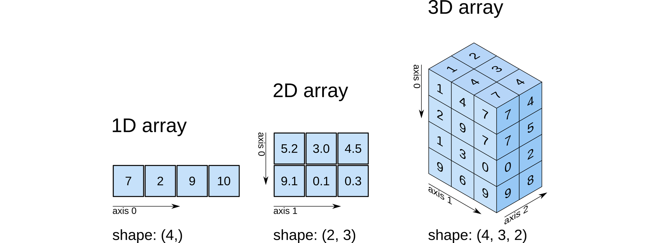
At the heart of NumPy is the NumPy array, which is used to store data into a structured format with multiple dimensions.
Depending on the dimensionality, these arrays correspond to our conventional notion of scalars (0D), vectors (1D), and matrices (2D), which is also described by their shape.
Each available dimension of the specific array is called an axis, which is how we index into them and it factors into certain calculations.
The figure below from O’Reilly illustrates these concepts:
Exercise: Creating NumPy arrays
There are many ways to create NumPy arrays, and we’ll demonstrate a few here. Print the following arrays to confirm that the output is correct (and note the formatting).
First create a NumPy array by converting a list of lists (the
numvariable below).Print the
typeof the original list and the new NumPy array to confirm they’re different.
Using NumPy, create the following 1D arrays:
A range of integers from 0 to 99, inclusive.
An array of 15 evenly-spaced numbers from 0 to 50, inclusive.
Then create the following 2D \(3 \times 3\) arrays using built-in NumPy functions:
A matrix of zeros.
A matrix of ones.
An identity matrix.
A diagonal matrix with
[1, 2, 3]along the main diagonal.A matrix of random numbers between \([0, 1)\).
Because NumPy is an external package, we have to first import it and then attach the prefix to its functions and modules. Example:
import numpy as np   # this is called an alias. Standard practice, saves our fingers. :)
np.ones(5)           # this creates a 5-element vector of 1's. Note the "np" alias.
np.random.rand()     # this creates a single random number between [0, 1) using np.random sub-module.
import numpy as np
num = [[1, 2, 3], [4, 5, 6]]
# -------------   WRITE YOUR CODE IN THE SPACE BELOW   ---------- #
Diffusion (Brownian motion)
On the surface, and particularly in the output, a NumPy array looks much like a list of lists (of lists of lists…)—how lame. But, once we get a true NumPy array, we can do some cool calculations with it. In particular, let’s assume we have some data representing random walk diffusion on a lattice, where our array is structured as follows:

Briefly, the data are generated using the following algorithm:
We start at the origin and each time step we randomly move forward or backward along one dimension in 3D space (hop to a nearest-neighbor lattice site).
We do this for a total of 100 time steps to get the first 2D array of data (where its shape is \(101 \times 3\)).
Then, we repeat the whole procedure 500 times (trials) to get a 3D array of data (where its shape is \(500 \times 101 \times 3\)).
While this is a relatively basic algorithm, it’s an instructive starting point for diffusion models and, in our case, scientific computing practice. The diffusion model could be for species on the surface of a catalyst, substitutional or interstitial atoms in an alloy, or ions in an electrolyte solution. In particular, it can be shown that the mean squared displacement (MSD) of such a particle from its original position \(\vec{x}_0\) is
where \(n\) is the dimensionality, \(t\) is the time, and \(D\) is the diffusion coefficient. Pretty neat!
Exercise: calculations along an axis
Your job will be to calculate the MSD using the diffusion data that we’ve loaded for you below.
The NumPy array is structured exactly as shown above (we can print data.shape to confirm this).
Your final answer should be a single array of length 101 with values that are approximately equal to:
[ 0. 1. 2. ... 99. 100.]
Hint: You might find the np.linalg.norm() and np.mean() functions helpful.
You will want to specify a specific axis parameter in each function.
Also, which function should you compute first?
data = np.load('../../assets/data/week_1/01/lattice_diffusion.npy')
print(f'The data has dimensions {data.shape}.')
# -------------   WRITE YOUR CODE IN THE SPACE BELOW   ---------- #
The data has dimensions (500, 101, 3).
More NumPy and linear algebra fun (aka machine learning??)
In the final set of problems, we’ll practice some more NumPy array operations in the context of a linear regression problem. Specifically, we will construct a linear model to predict the atomic weight of an element using its atomic number. You know from your previous studies that the two properties are related:
but not perfectly linear, which makes this a good problem for demonstrating the method of least squares. If you need a reminder of the matrix-vector formulation of the least squares regression problem, see this handout or similar ones on Google.
Exercise: solve an ordinary least squares problem using the normal equation
We have provided some data for you in number_weight.npy (loaded below) with 50 rows and 2 columns.
The first column is the atomic number and the second column is the atomic weight for the corresponding element.
Your job is to create a design matrix \(X\) that consists of the following columns:
A column of ones.
A column of atomic numbers.
A column of atomic numbers squared (this is an example of adding polynomial features, which we’ll discuss on Thursday).
You should also create a target vector \(\vec{y}\) that is the column of atomic weights. To be even more explicit, your code should do the following:
After this is done, you should compute the regression coefficients (weights) \(\vec{\theta}\) using the normal equation:
where \(\vec{\theta}\) is such that for the \(i\)th element (i.e., \(i\)th row of \(X\)),
Finally, compute the root-mean-square error (RMSE), which is given by
If you print out your \(\vec{\theta}\) values and RMSE, you should get approximately
Hint: You may want to use np.column_stack() (or see np.concatenate() for more options), np.linalg.inv(), ndarray.T, np.matmul() (or simply the @ operator), and the np.linalg.norm() function.
data = np.load('../../assets/data/week_1/01/number_weight.npy')
# -------------   WRITE YOUR CODE IN THE SPACE BELOW   ---------- #
Exercise: last one!
We’ll conclude with another conceptual exercise. Enze receives some measurement data with recorded temperature values. He quickly realizes that his collaborators recorded the data in degrees Celsius instead of Kelvin, so he has to add \(273\) to his data and writes the following code to do so. Explain what the following code would do and why this is very dangerous! Try to first answer the question without actually running the code. 😉
A = np.array([[1, 2, 3], [4, 5, 6]])   # this creates a 2x3 array
B = 273 * np.ones(3)                   # this creates a 1x3 array
C = A + B                              # what will happen here??
Answer: ____
Conclusion
Congratulations on completing these exercises! 🎉👏
These problems were definitely not easy and it’s OK if you need a little more time to digest everything we covered above.
Please don’t hesitate to reach out on Slack if you have questions or concerns.