Tabular data¶

Authors: Enze Chen and Mark Asta (University of California, Berkeley)

Note

This is an interactive exercise, so you will want to click the and open the notebook in DataHub (or Colab for non-UCB students).

Learning objectives¶

This notebook contains a series of exercises that explore tabular data and the pandas package. We hope that after going through these exercises, you will be prepared to:

Follow best practices for structuring data into a tabular format.
Use pandas and other programmatic tools to operate tabular data.
Perform some exploratory data analysis (EDA) to gain insights about your data.

Contents¶

These exercises are grouped into the following sections:

CSV files
pandas!
Formatting tabular data
Procuring tabular data

CSV files¶

Back to top

In the previous exercise, we came across a CSV file with the following data:

# Data obtained from Wikipedia
Element,Number,Mohs hardness,Density (g/cc)
lithium,3,0.6,0.534
beryllium,4,5.5,1.85
boron,5,9.4,2.34
carbon,6,10,3.513
...

and we noted that this data had structure to it (not just arbitrary text characters). Specifically, each row after the second has comma-separated tokens that are intuitively represented as str, int, float, and float, corresponding to the terms in the second row. Now, you may already know that CSV stands for “comma-separated values,” but even if you didn’t know this, you probably knew that CSV files are typically opened in an application like Microsoft Excel or Google Sheets, generating a tabular representation of the data. It turns out that these programs are specially designed to handle CSV files by splitting the data into cells based on the presence of commas. They try to do this with any file that ends in .csv, which is why in the previous exercise we mentioned that operating systems with GUIs benefit from having the “correct” file extension, even though a CSV is just a plain ol’ text file.

Wait, but what about Excel files?¶

So if you’ve used Microsoft Excel, you may be familiar with their .xls or .xlsx file formats that also store tabular data. In fact, if you’ve ever modified a .csv file in Excel and then tried to save it, you may have even seen a warning informing you that you should save the data as an Excel file to avoid loss of information (such as preservation of formulas, having multiple sheets in one file, etc.). While some of these Excel features are nice, the file format is less so, and can be quite difficult to process programmatically and is often not cross-platform compatible (even Windows vs. Mac versions of Excel can conflict with each other!), which is not a good practice in MI. Therefore, we recommend that you choose to store tabular data in CSV instead of native Excel, at least when working with your peers in this module.

Why do we want tabular data?¶

CSV data are typically rendered in tabular form to easily identify the association between variables, whether we’re associating all the values in a row, or the value at a particular row-column location. They provide a concise summary of the data, without using many words, so that general trends can be surfaced at a glance. We can quickly perform statistical analyses of groups (i.e., columns) of data, which you may have done with the =AVERAGE() or =SUM() functions in Excel. It’s also easy to create data visualizations when data are in a table, such as plotting \(y\)-values against \(x\)-values, and we’ll see more examples of this tomorrow!

While there are many more advantages (and disadvantages!) one could list for tabular data, we still have yet to discuss how to get our data into a table so that we can access these benefits. In the previous notebook, we tried reading in the above file as a list of lists and as a NumPy array, which gave

[['lithium', 3, 0.6, 0.534],
 ['beryllium', 4, 5.5, 1.85],
 ['boron', 5, 9.4, 2.34],
 ['carbon', 6, 10.0, 3.513],
 ...
]

and

array([['lithium', '3', '0.6', '0.534'],
       ['beryllium', '4', '5.5', '1.85'],
       ['boron', '5', '9.4', '2.34'],
       ['carbon', '6', '10.0', '3.513'],
       ...
      ])

respectively. Neither seem like great options, as the former is tricky to take vertical slices of and the latter is all strings. Moreover, it took a few lines of Python to even get the data loaded in the first place, which seems clunky. 😓 Motivated by our experience with JSON files, it would be great if we could load in the entire file into a tabular form that preserves individual data types in each column…

pandas!¶

Back to top

pandas

Luckily, our furry friends from the East 🐼 have heard our pleas and are here to save the day! …kinda. Not really.

pandas is Python package developed in 2008 by Wes McKinney to facilitate data analysis and it has since become one of the most widely used packages in the Python community. The name is cleverly derived from “panel data,” which is a phrase from econometrics for “multi-dimensional time series” and is the context for which pandas was first developed. pandas is built on top of NumPy, so there are many aspects of it that you should already be familiar with!

`DataFrame` and `Series`¶

At the heart of pandas lies two data structures for all of your informatics needs.

The DataFrame follows our conventional notion of a spreadsheet for 2D tabular data. Note that a DataFrame is for 2D data only and does not work for lower or higher dimensions (unlike NumPy arrays). They feature row and column labels for intelligent indexing and they support heterogeneously-typed columns. 🙌
Each column of a DataFrame is a Series, which is a 1D array with axis labels. Note that a Series is homogeneously-typed.

`DataFrame` constructor¶

The best way to learn is by doing, so let’s go ahead and use pandas to construct a DataFrame.

The community standard is to use the alias

import pandas as pd 

which is similar to using np for numpy, so it’s best practice to stick with this alias. Or else people might look at you like 🤨.

There are many ways to create DataFrames, but with the DataFrame() constructor you will likely use one of two methods:

pd.DataFrame(dict), where dict is a dictionary of str:list pairs that correspond to the name and values in each column.
pd.DataFrame(arr, columns=col_names), where arr is a 2D NumPy array or list of lists and col_names are the names you want to assign each column.

Let’s see this in practice.

import pandas as pd    # note alias

# Create a DataFrame from dict
df_dict = pd.DataFrame({     # we split onto many lines for ease of reading
    'symbol': ['H', 'He', 'Li'],
    'number': [1, 2, 3],
    'mass': [1.008, 4.003, 6.941]
})
print(df_dict)

# Create the same DataFrame from list of lists
df_list = pd.DataFrame([['H', 1, 1.008], ['He', 2, 4.003], ['Li', 3, 6.941]],
                       columns=['symbol', 'number', 'mass'])
display(df_list)    # in Jupyter notebooks, DataFrames have a pretty display (compare to print above)

  symbol  number   mass
    H       1  1.008
   He       2  4.003
   Li       3  6.941

	symbol	number	mass
0	H	1	1.008
1	He	2	4.003
2	Li	3	6.941

Using the constructor directly is a common approach when you’re trying to create a DataFrame from non-tabular data sources, so you might see yourself using this method in your own work if you’re scraping together data from text files or databases.

But what if your data source is a CSV file that’s already nicely formatted for you? As with our first example in this notebook, it would be nice if we could directly use that structure and express it in Python. To do this, we will use the pd.read_csv() function which does exactly as the name describes. This function, as you can see from the documentation, has a bajillion input arguments that we don’t have time to cover today, so we’ll describe just a few here:

filepath_or_buffer: The only required argument, which is the file you’re trying to read in.
sep: The character separating your data tokens. Default is comma (','), but you can change this to be space (' '), tab ('\t'), etc.
header: Which row to read column headers from. Default is the first row.
names: If you would like to rename your columns. This list cannot have duplicates.
skiprows: Extremely useful if there are lines of comments and extra text at the top of the file that you want to avoid reading.
nrows: Useful if your file is very large, or your data stops before reaching the end of the file (e.g., there’s footer text in the file).

Reading in a CSV file¶

Let’s use pd.read_csv() to read in our hardness_density.csv file! We’ll save the DataFrame into a variable called df. This isn’t great practice because our variable names should be descriptive, but for this tutorial it’s an easy reminder of what we’re working with and saves our fingers some work. We’ll also rename the column names to be:

['element', 'number', 'hardness', 'density']

which can do if we set header=0.

df = pd.read_csv('../../assets/data/week_1/02/hardness_density.csv', sep=',', skiprows=1,  # skip comment line
                 header=0, names=['element', 'number', 'hardness', 'density'])   # we rename for simplicity
df

	element	number	hardness	density
0	lithium	3	0.60	0.534
1	beryllium	4	5.50	1.850
2	boron	5	9.40	2.340
3	carbon	6	10.00	3.513
4	sodium	11	0.50	0.968
5	magnesium	12	2.50	1.738
6	aluminium	13	2.75	2.700
7	silicon	14	6.50	2.330
8	sulfur	16	2.00	2.080
9	potassium	19	0.40	0.890
10	calcium	20	1.75	1.550
11	titanium	22	6.00	4.506
12	vanadium	23	7.00	6.110
13	chromium	24	8.50	7.150
14	manganese	25	6.00	7.210
15	iron	26	4.00	7.860
16	cobalt	27	5.00	8.900
17	nickel	28	4.00	8.908
18	copper	29	3.00	8.960
19	zinc	30	2.50	7.140
20	gallium	31	1.50	5.910
21	germanium	32	6.00	5.323
22	arsenic	33	3.50	5.727
23	selenium	34	2.00	4.810
24	rubidium	37	0.30	1.532
25	strontium	38	1.50	2.640
26	zirconium	40	5.00	6.520
27	niobium	41	6.00	8.570
28	molybdenum	42	5.50	10.280
29	ruthenium	44	6.50	12.450
30	rhodium	45	6.00	12.410
31	palladium	46	4.75	12.023
32	silver	47	2.50	10.490
33	cadmium	48	2.00	8.650
34	indium	49	1.20	7.310
35	tin	50	1.50	7.265

And there’s all of our data! That was pretty efficient. To see all of the input/output functions available to you, we point you to the documentation.

The takeaway here is that, like the json package, we’re using the pandas package because that is the most convenient way to process this particular structure of data, and the fastest way to get us what we want.

Working with DataFrames¶

We got our data into a DataFrame! Now what?

Well, now the fun begins. 😄 Note: A lot of the following discussion is centered around DataFrames, but many of the attributes/methods apply to Series as well.

The first thing you might be interested in is the dimensions of your data (DataFrame). We can access that using the df.shape attribute. Again, attributes in Python don’t have parentheses; only methods (i.e., functions) do!

df.shape

(36, 4)

Not bad, just like NumPy. 😉 Note that the column name/header is not part of the “data itself,” which probably aligns with your intuition and we’re just pointing it out for good measure.

Try it out: What does the related attribute df.size do?

If you just want the list of column names, you can get (and set!) them using the df.columns attribute.

df.columns

Index(['element', 'number', 'hardness', 'density'], dtype='object')

How about the data types in the DataFrame? We claimed that DataFrames are heterogeneously-typed (different columns (Series) can hold different data types) but the proof is in the pudding, which in this case is the df.info() method.

df.info()

<class 'pandas.core.frame.DataFrame'>
RangeIndex: 36 entries, 0 to 35
Data columns (total 4 columns):
 #   Column    Non-Null Count  Dtype  
---  ------    --------------  -----  
 0   element   36 non-null     object 
 1   number    36 non-null     int64  
 2   hardness  36 non-null     float64
 3   density   36 non-null     float64
dtypes: float64(2), int64(1), object(1)
memory usage: 1.2+ KB

Pause and reflect: Is the above information what you would expect to see?

Five-number summary and exploratory data analysis¶

When starting out with any data-driven methodology, it is a good idea to perform some elementary statistical analysis on your dataset to get a sense of the distribution, presence of outliers/holes, etc. This procedure is termed exploratory data analysis (EDA) and often involves generating plots of your data, so we’ll be doing more of it during tomorrow’s data visualization lessons.

There are, however, also some simple numerical tests you can run, such as checking for NaN values with the df.info() method from above (see third column). Another set of descriptive statistics that is helpful to compute is the five-number summary for the percentiles in your sample. In pandas, we can easily do this by calling the df.describe() method.

df.describe()

	number	hardness	density
count	36.000000	36.000000	36.000000
mean	28.166667	3.990278	5.809639
std	14.035669	2.605730	3.536701
min	3.000000	0.300000	0.534000
25%	18.250000	1.937500	2.337500
50%	28.500000	3.750000	6.010000
75%	40.250000	6.000000	8.590000
max	50.000000	10.000000	12.450000

You may have noticed that the 'element' column was ignored because that Series has a non-numeric type. It is still possible to get statistics on that Series if we single it out. We can select a single column by creating a length 1 list with just that column name, which returns a DataFrame object.

df[['element']].describe()   # More on indexing in a bit!

	element
count	36
unique	36
top	nickel
freq	1

You can also calculate a specific summary statistic using the appropriate method (which typically has an axis parameter that you can specify).

df.mean(axis=0)   # axis=1 gets the mean of the rows

number      28.166667
hardness     3.990278
density      5.809639
dtype: float64

To see the number of unique entries in a column (mostly for categorical data), we can use the df.nunique() method.

df.nunique()

element     36
number      36
hardness    22
density     36
dtype: int64

Another way to check data distribution for categorical variables is through the df.value_count() method.

df['hardness'].value_counts()   # not super exciting because this is a real-value variable

00     5
50     3
50     3
00     3
50     2
00     2
00     2
50     2
50     1
20     1
60     1
75     1
30     1
50     1
75     1
00     1
00    1
40     1
00     1
40     1
50     1
75     1
Name: hardness, dtype: int64

Making heads or tails of DataFrames¶

You may have noticed that when we display a DataFrame, we get quite a lot of rows. But maybe in some cases we don’t really need to see all the rows, which quickly fills up our Jupyter workspace. The df.head(n) method will return the first \(n\) (default is 5) rows of your DataFrame, and is commonly used to check that column headers and first few values are correctly loaded in. The df.tail(n) method works analogously, but for the last \(n\) rows.

df.head()

	element	number	hardness	density
0	lithium	3	0.6	0.534
1	beryllium	4	5.5	1.850
2	boron	5	9.4	2.340
3	carbon	6	10.0	3.513
4	sodium	11	0.5	0.968

Exercise: display the last 10 rows of the DataFrame¶

# -------------   WRITE YOUR CODE IN THE SPACE BELOW   ---------- #

There will also be times where you do want to see more columns and rows than what Jupyter allows by default. In those cases, we point you to use the suggestion in this Stack Overflow post. Don’t worry—it’s a safe practice, we’re just making you work for your meal. 😁

We can also sort the values in a DataFrame using the df.sort_values() method, which takes a single string or a list of strings for the columns we want to sort by. A copy of those values is then returned.

df.sort_values('density').head()

	element	number	hardness	density
0	lithium	3	0.60	0.534
9	potassium	19	0.40	0.890
4	sodium	11	0.50	0.968
24	rubidium	37	0.30	1.532
10	calcium	20	1.75	1.550

Indexing and slicing a DataFrame¶

There are many ways to index into a DataFrame and slice it to get subsets of your data. If we want to get the data in a particular column, we can get the Series using the column name, much like how we would use the key in a dictionary:

hardness = df['hardness']
print(type(hardness))
print(f'Shape: {hardness.shape}')
hardness.head()

<class 'pandas.core.series.Series'>
Shape: (36,)

   0.6
   5.5
   9.4
  10.0
   0.5
Name: hardness, dtype: float64

Try it out: What happens if you wrote df[['hardness']] above instead?

To select multiple columns, use a list of column names within brackets [].

multiple = df[['hardness', 'density']]
print(type(multiple))
multiple.head()

<class 'pandas.core.frame.DataFrame'>

	hardness	density
0	0.6	0.534
1	5.5	1.850
2	9.4	2.340
3	10.0	3.513
4	0.5	0.968

We can perform Boolean indexing as follows, combining logical operators as needed (must use |/& instead of or/and):

df[df['hardness'] > 8.0]

	element	number	hardness	density
2	boron	5	9.4	2.340
3	carbon	6	10.0	3.513
13	chromium	24	8.5	7.150

df[(df['hardness'] > 8.0) & (df['density'] < 5.0)]

	element	number	hardness	density
2	boron	5	9.4	2.340
3	carbon	6	10.0	3.513

To get slices of the data, particularly when we only want a subset of the rows, we do this in two different ways:

The df.loc[] property accesses data by labels (mostly) or Boolean arrays (sometimes).
The df.iloc[] property accesses data based on the integer index position.

Note that these are square brackets! Which one you choose to use depends on your use case. In some of the previous examples, you may have noticed that even after the DataFrame got shuffled, the bold row labels were preserved. These are labels one would use for the loc[] property, for example, and we demonstrate this below.

df_sub = df.sort_values('density').head(10)
df_sub    # a subset of values is easier to work with

	element	number	hardness	density
0	lithium	3	0.60	0.534
9	potassium	19	0.40	0.890
4	sodium	11	0.50	0.968
24	rubidium	37	0.30	1.532
10	calcium	20	1.75	1.550
5	magnesium	12	2.50	1.738
1	beryllium	4	5.50	1.850
8	sulfur	16	2.00	2.080
7	silicon	14	6.50	2.330
2	boron	5	9.40	2.340

df_sub.loc[:, 'hardness']    # a column

   0.60
   0.40
   0.50
  0.30
  1.75
   2.50
   5.50
   2.00
   6.50
   9.40
Name: hardness, dtype: float64

df_sub.loc[[0, 9, 7], ['hardness', 'number']]    # labels can be in any order

	hardness	number
0	0.6	3
9	0.4	19
7	6.5	14

df_sub.loc[:10, ['hardness', 'density']]    # a chunk subset

	hardness	density
0	0.60	0.534
9	0.40	0.890
4	0.50	0.968
24	0.30	1.532
10	1.75	1.550

We want to point out two things about the previous example:

Note that we’re saying “take all the row indices up to the label value 10,” not the 10th position! Try changing the above value to 6 and see what happens.
Note that in pandas, unlike Python/NumPy, the upper bound is inclusive.

Those examples were with df.loc[]. Now for df.iloc[]:

df_sub.iloc[:4, :2]    # a chunk subset

	element	number
0	lithium	3
9	potassium	19
4	sodium	11
24	rubidium	37

df_sub.iloc[:, 1]    # a column of values

    3
   19
   11
  37
  20
   12
    4
   16
   14
    5
Name: number, dtype: int64

df_sub.iloc[0, 3]    # a single value

0.534

Looping through a DataFrame¶

While a DataFrame supports really clever and advanced indexing, there will be times when, for lack of a better method, we simply need to iterate through a DataFrame and access the entries one row/column at a time. If you disagree with us, or want to know why one would disagree, please see this Stack Overflow discussion. 😛

If you want to loop over the rows (more common than looping through columns, simply based on our formatting conventions), the preferred method is df.itertuples(), which returns an iterator over the rows as named tuples. Note that by default, the index of the rows is the first element of the tuple, followed by the other elements in the row.

for row in df_sub.itertuples():
    print(row)           # the full row
    print(row.element)   # how we access the values by name
    print(row[2])        # access by integer index
    if row[0] > 10:
        break            # early stopping; we get the idea

Pandas(Index=0, element='lithium', number=3, hardness=0.6, density=0.534)
lithium
3

Pandas(Index=9, element='potassium', number=19, hardness=0.4, density=0.89)
potassium
19
Pandas(Index=4, element='sodium', number=11, hardness=0.5, density=0.968)
sodium
11
Pandas(Index=24, element='rubidium', number=37, hardness=0.3, density=1.532)
rubidium
37

Updating a DataFrame¶

There are many times when we will want to update the DataFrame that we created. This could be for:

Adding additional columns based on a computation.
Changing the values for a particular use case.
Merging several DataFrames together.

Let’s see a few examples of this right now. We’ll start by adding on two columns, which we can do as if we’re defining a new dictionary entry. Just ensure that the additional columns have the same size as the number of rows in the DataFrame.

import numpy as np
df['ones'] = np.ones(len(df))   
df['number_squared'] = df['number'] ** 2   # we can perform arithmetic on other columns
df.head()

	element	number	hardness	density	ones	number_squared
0	lithium	3	0.6	0.534	1.0	9
1	beryllium	4	5.5	1.850	1.0	16
2	boron	5	9.4	2.340	1.0	25
3	carbon	6	10.0	3.513	1.0	36
4	sodium	11	0.5	0.968	1.0	121

We can eliminate columns/rows of our DataFrame using the df.drop() method on the labels we wish to drop. Note that by default a copy of the resulting DataFrame is created. In addition, the row labels that may have been automatically indexed initially (with a RangeIndex) will not be reindexed automatically, so we might want to call the df.reset_index() method on the DataFrame.

df_smaller = df.drop(df[df['density'] > 1.0].index)   # putting it all together!
display(df_smaller)

df_smaller = df_smaller.reset_index(drop=True)   # arg prevents original index from being inserted as new column
df_smaller                                       # note how indices on far left are reset

	element	number	hardness	density	ones	number_squared
0	lithium	3	0.6	0.534	1.0	9
4	sodium	11	0.5	0.968	1.0	121
9	potassium	19	0.4	0.890	1.0	361

	element	number	hardness	density	ones	number_squared
0	lithium	3	0.6	0.534	1.0	9
1	sodium	11	0.5	0.968	1.0	121
2	potassium	19	0.4	0.890	1.0	361

Undefined values¶

Now let’s see what happens if our data has “holes,” and how we can use built-in pandas functions to change those values. pandas represents missing data with the NumPy constant np.nan. In the example below we’re setting values to be NaN, but if you were to read in a CSV with missing values, then those positions would also contain NaN.

df_holey = pd.DataFrame(np.arange(15).reshape(3, 5))
df_holey.iloc[:, -1] = np.nan   # set last column to be NaN
df_holey.iloc[0, 0] = np.nan    # set first element to be NaN
print(df_holey.dtypes)
df_holey

  float64
    int32
    int32
    int32
  float64
dtype: object

	0	1	2	3	4
0	NaN	1	2	3	NaN
1	5.0	6	7	8	NaN
2	10.0	11	12	13	NaN

As a first step, we might want to know where the NaN values are, or to get a mask for post-processing. We can do this using the df.isna() method, which returns a Boolean DataFrame that is True for NaN cells and False otherwise.

df_holey.isna()

	0	1	2	3	4
0	True	False	False	False	True
1	False	False	False	False	True
2	False	False	False	False	True

To remove rows or columns of the DataFrame with NaN values, we can use the df.dropna() method, which typically needs the following parameters specified (i.e., don’t just use the default):

axis: 0 for index, 1 for columns.
how: any if that dimension has any NaN values, all if that dimension has all NaN values.

df_holey.dropna(how='any', axis=1)   # what got dropped? what happens if axis=0? what if how='all'?

	1	2	3
0	1	2	3
1	6	7	8
2	11	12	13

We can also fill in the NaN values with a default value that often depends on the application. For example, if we have data on processing times, then a blank value might indicate that process was never performed; or, alternatively, performed for 0 time units. Filling in data in this way is called imputation and must be done with care to not bias the data or follow-up analyses. Filling in NaN values can be done with the df.fillna() method, which is quite flexible.

df_holey.fillna(value=0.0)

	0	1	2	3
0	0.0	1	2	3
1	5.0	6	7	8
2	10.0	11	12	13

Saving a DataFrame¶

We’ve discussed how to read in CSV file as a DataFrame, so how can we do the reverse to save our work? The df.to_csv() method will do this job perfectly. Like its counterpart, pd.read_csv(), there are a ton of input arguments to this method, but arguably the three most important ones are:

path_or_buf: The filepath where you want to store the CSV file.
index: Whether to include a column for the row indices. Default is True, but you should probably set this to False.
sep: What delimiter to use to separate values. Default is comma (','), which probably doesn’t need to change (unless your DataFrame’s values have commas in them).

df_holey.to_csv('../../assets/data/week_1/02/df_holey.csv', index=False)

Formatting tabular data¶

Back to top

In all of our discussion so far, we’ve somewhat casually mentioned ideas like “Oh, now we should average all the values in the column,” or “Now take the norm of each row,” without really motivating why our data might be arranged in that way to begin with. Like with many other things in life, there are certain formatting conventions when it comes to tabular data, and we’ll take some time to discuss those right now. For example, given the same set of data, I could conceivably store it in a spreadsheet (CSV file) in the following two ways:

table format

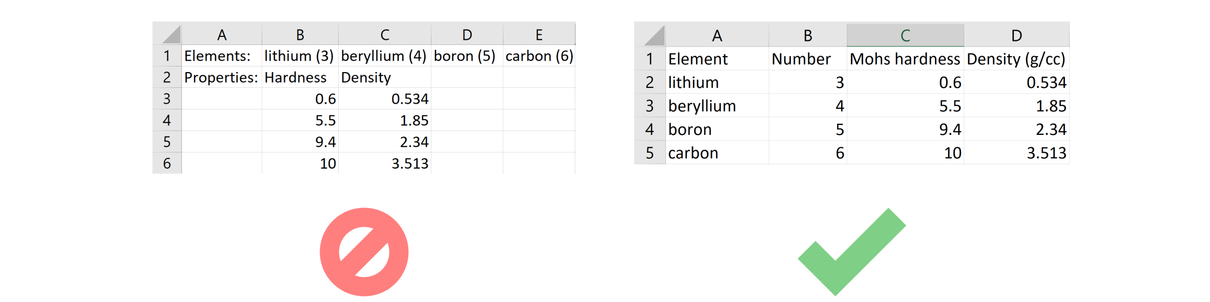
Now, if you’re looking at the image on the left and thinking, “Pshht, there’s no way anyone would ever do that,” then you are lucky to have great collaborators. 😜 In any case, the spreadsheet on the left does not have a uniform structure for accessing the data, which can make it tricky to perform statistical analyses or even figure out which values are meant to be associated. The image on the right is much more preferred for data science because each row is a distinct entry and each column is a different property of that entry that is clearly labeled. In short, the convention for formatting tabular data for MI is:

Each row should be a single example (data point), whether that is data collected from a different material, a different site, or at a different time.
Each column should be a single property, or feature, associated with the data point. In the example above, this would be the element name, number, hardness, and density.

Please don’t get rows and columns transposed!

Exercise (conceptual): CSV vs. JSON 🥊¶

Based on what you’ve seen so far, what are the advantages of CSV over JSON, and vice versa? Please record your thoughts somewhere and we’ll discuss this question later!

Exercise: Reformatting dielectric constants dataset¶

The Strehlow and Cook dataset you saw in the last notebook was pretty complex partially because it was compiled from a variety of disparate sources, so in this example we will work with a cleaner dataset from Petousis et al., Scientific Data, 2017. The data from their work is featured in the overview figure for this module and it is shared as a JSON file in the Dryad repository.

We’ve downloaded the dataset here for you as dielectric_dataset.json and your job is to take this JSON of 1056 materials and extract each material’s:

Materials Project ID (has a value like mp-XXX)
chemical formula
refractive index, \(n\)
band gap, \(E_g\)
total dielectric constant, \(\varepsilon_{\text{poly}}\)
electronic contribution to the dielectric constant, \(\varepsilon_{\text{poly}}^{\infty}\)

and organize this information into an appropriate pandas DataFrame. Finally, save this DataFrame as a CSV file in a location where you can find it again. You might need the tabular version of this dataset in future exercises and research work, just so you know. 😁

Hints:

You should open the file on your computer, or print out the first element in data using Python code, to see what the appropriate keys and access patterns should be.
You may assume that every material has every property that’s listed above and that each JSON entry is formatted the same way. Recall that this wasn’t true for Strehlow and Cook, but that’s the benefit of using computational data like these.
You may want to display the final DataFrame when you’re done, just to confirm that you got all the data you needed (correct dimensions, columns, values, etc.).

import json
with open('../../assets/data/week_1/02/dielectric_dataset.json', 'r') as f:
    data = json.load(f)
# -------------   WRITE YOUR CODE IN THE SPACE BELOW   ---------- #

Procuring tabular data¶

Back to top

For the final segment of this lesson, we will discuss some other software (outside of the Python ecosystem) that can help us obtain tabular data (i.e., in a CSV format) from sources that are almost, but not quite tabular.

WebPlotDigitizer¶

For example, from Module 1, you all looked at the recent paper by Wu et al. J. Micro/Nanopatterning, 2021 (in Google Drive) where Figure 1 plotted dielectric constant vs. refractive index for a few alloys. This is a nice plot, as are many other plots in published papers, but how can we extract the numerical values from these figures?

WebPlotDigitizer is a common tool for this purpose. In the web application, you upload an image file (such as a plot) and you can mark \(x\) and \(y\) coordinates that get estimated and turned into a CSV file for you. Originally we were planning a small exercise for you to practice with this, but we’ll leave it up to you to decide if this is worth exploring for your own self-directed research.

Tabula¶

Relatedly, published papers and reports will often feature several nice tables… that are stuck in PDFs. If the PDF is relatively modern, maybe you can copy-paste the information out from there and into a spreadsheet application. But if the PDF is old or of poor quality (such as many scanned documents), you’ll be left with a dingy table that you have to manually copy the data out by hand… or do you?

Tabula is a tool that was designed to solve this problem, although it is no longer under active development. With this tool, you can upload a PDF file, select the tables inside it, and then the software will attempt to “read” the selection and convert the table into a CSV file. There will likely be a few errors here and there, but you might find that this saves you a lot of trouble if you have a lot of PDF-embedded tables to parse!

Manual entry¶

It’s possible that at the end of the day, you still have to enter data into CSV files by hand. And that’s OK! There are pros and cons of taking this route, and since we are teaching you programmatic tools for MI (and benefits like automation, reproducibility, etc.) we haven’t really talked about this, but we definitely don’t want you to think this is off limits. Sometimes, it’s about using whatever gets the job done. 😆

Conclusion¶

This concludes the introduction to tabular data. If you would like to learn more about pandas, we suggest you look at the official user guide. Realistically, there’s way too much to cover about pandas, and a lot of your understanding will be built as you work with it for your own datasets. But, we hope that by giving a brief introduction, you at least know what’s available, where to go for help, and how to think about tabular data with pandas.

For the final notebook lesson of the day, we’ll be learning about databases and the Materials Project!

Introduction to Materials Informatics

Tabular data¶

Learning objectives¶

Contents¶

CSV files¶

Wait, but what about Excel files?¶

Why do we want tabular data?¶

pandas!¶

DataFrame and Series¶

DataFrame constructor¶

Reading in a CSV file¶

Working with DataFrames¶

Five-number summary and exploratory data analysis¶

Making heads or tails of DataFrames¶

Exercise: display the last 10 rows of the DataFrame¶

Indexing and slicing a DataFrame¶

Looping through a DataFrame¶

Updating a DataFrame¶

Undefined values¶

Saving a DataFrame¶

Formatting tabular data¶

Exercise (conceptual): CSV vs. JSON 🥊¶

Exercise: Reformatting dielectric constants dataset¶

Procuring tabular data¶

WebPlotDigitizer¶

Tabula¶

Manual entry¶

Conclusion¶

`DataFrame` and `Series`¶

`DataFrame` constructor¶