Example 2-2: Quiver plots

Important!

If you’re completely new to Python, you may want to go through the exercises in the Python fundamentals notebook first!

Note

Click the and open this notebook in Colab to enable interactivity. We encourage you to experiment with customized values to deepen your learning.

Note

To save your progress, make a copy of this notebook in Colab File > Save a copy in Drive and you’ll find it in My Drive > Colab Notebooks.

While the majority of this class will be spent on solving ordinary differential equations (ODEs) analytically and numerically, a key aspect of verifying the correctness of our solution is by plotting it. In this example, we will show how to make arrow plots that represent the direction field in a region (you may have seen these plots in the context of vector fields in CME 100).

Summary of commands

In this exercise, we will demonstrate the following:

• Numpy

  • np.linspace(start, stop, num) - Returns num evenly spaced numbers between start and stop (inclusive).

  • np.meshgrid(x, y) - Create a 2D grid of coordinate values based on 1D x and y arrays.

    • The result is two X and Y 2D arrays with the corresponding 1D arrays tiled across the other dimension.

  • np.ones(shape) - Returns an array of the given shape of all 1s.

  • Common functions like np.sqrt(x) and np.exp(x) for \(\sqrt{x}\) and \(e^{x}\), respectively, of an array x (element-wise).

• Matplotlib

  • plt.subplots() - Create Figure and Axes objects for plotting. Many possible parameters.

  • ax.quiver(X, Y, U, V) - Plot a field of arrows at the given locations X,Y pointing in U,V.

  • ax.plot(x, y, ...) - Create a scatter/line plot in 1D, y vs. x. Many styles possible.

  • ax.set(...) - Set axes xlabel, ylabel, xlim, ylim, title, etc.

Direction field

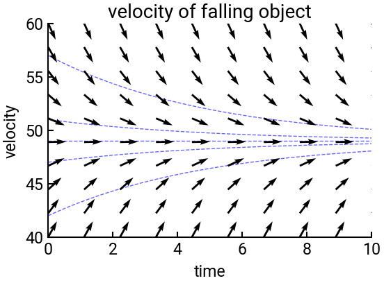
An object of mass \(m\) is dropped with an initial velocity \(v_0\), and is falling under the force of gravity (constant acceleration \(g\)) and the effect of air friction. It is our desire to find an ODE governing the velocity \(v(t)\) of the object.

It can be shown that the governing ODE and its initial conditions are:

\[ \frac{dv}{dt} = - \frac{\gamma}{m} v + g; \qquad v(0) = v_0 \]

Now we’ll create a direction field plot for the range \(0 \le t \le 10\) and \(40 \le v(0) \le 60\). This leverages the ax.quiver() command to plot arrows over a np.meshgrid() of points. We will also superimpose the exact solutions (you can verify this to be

\[ v = \frac{g}{K} + \left( v_0 - \frac{g}{K} \right) \exp \left( -K t \right) \]

through direct integration, where \(K = \dfrac{\gamma}{m}\)) and add some informative plot styling.

# import libraries
import numpy as np
import matplotlib.pyplot as plt

# constants
g = 9.8
K = 0.2

# set up grid w/ limits
t = np.linspace(0, 10, 10)
y = np.linspace(40, 60, 10)
[T, Y] = np.meshgrid(t, y)

# create arrays for arrows - see course reader for details
v_t = np.ones(T.shape)    # set t-component of all vectors to 1
v_y = -K * Y + g          # calculate y-component
v_len = np.sqrt(v_t**2 + v_y**2)   # calculate vector length
v_t = v_t / v_len         # normalize
v_y = v_y / v_len         # normalize

# draw plot
fig, ax = plt.subplots()
ax.quiver(T, Y, v_t, v_y)
ax.set(xlabel='time', ylabel='velocity', title="velocity of falling object", 
       xlim=[0, 10], ylim=[40, 60])

# plot exact solutions with specific initial positions
y0 = [42, 47, 49, 51, 57]
t2 = np.linspace(0, max(t), 1000)
for yi in y0:
    y2 = g / K + (yi - g / K) * np.exp(-K * t2)
    ax.plot(t2, y2, 'b--', lw=1, alpha=0.6, zorder=-5)
plt.show()