Example 12-1: Dirichlet boundary conditions

So far we’ve only solved initial value problems where conditions are prescribed at the left end of the solution interval, i.e., at \(t = 0\). When conditions are prescribed for both ends of the solution interval, we get a boundary value problem (BVP), which we will explore in this section. We begin with defining a few different classes of BVPs and direct methods for solving them.

Summary of commands

In this exercise, we will demonstrate the following new commands:

• np.diag(x, k) - Construct a diagonal 2D array from the 1D array x, placing it on the kth diagonal.

  • Note: The main diagonal (\(a_{11}\), \(a_{22}\), \(a_{33}\), …) is \(k=0\). \(k > 0\) is above and \(k < 0\) is below.

• np.ones(shape) - Create an array of the given shape of all 1s.

• np.linalg.solve(A, b) - Computes the solution \(\vec{x}\) to the matrix equation \(A \vec{x} = \vec{b}\).

  • Note: This is the NumPy analog of the classic MATLAB expression x = A \ b.

• np.concatenate([M1, M2, ...], axis) - Join a sequence of arrays M1, M2, … along the given axis. Array dimensions must be consistent.

• ax.annotate(text, xy, ...) - Place the text string at the position xy.

  • Many other options available! Read more for details.

Direct methods

The idea behind direct methods is to use a finite difference scheme to discretize the derivatives, transforming a calculus problem into a linear algebra one. (fun!) The resulting matrix equation can then be solved using standard linear algebra tools in a single operation (“directly”). The tricky thing is setting up the coefficients in the A matrix and remembering to enforce the proper boundary conditions.

Because the discretization of derivatives only accounts for neighboring points, the general structure of these problems looks like the following:

\[\begin{split} \begin{pmatrix} b_2 & c_2 & \ & \ & \ & \ & \ \\ a_3 & b_3 & c_3 & \ & \ & \ & \ \\ \ & a_4 & b_4 & c_4 & \ & 0 & \ \\ \ & \ & \ddots & \ddots & \ddots & \ & \ \\ \ & 0 & \ & a_{N-3} & b_{N-3} & c_{N-3} & \ \\ \ & \ & \ & \ & a_{N-2} & b_{N-2} & c_{N-2} \\ \ & \ & \ & \ & \ & a_{N-1} & b_{N-1} \end{pmatrix} \begin{pmatrix} y_2 \\ y_3 \\ y_4 \\ \vdots \\ y_{N-3} \\ y_{N-2} \\ y_{N-1} \end{pmatrix} = \begin{pmatrix} f_2 \\ f_3 \\ f_4 \\ \vdots \\ f_{N-3} \\ f_{N-2} \\ f_{N-1} \end{pmatrix} \end{split}\]

The large coefficient matrix is tridiagonal, and we can easily construct it by specifying the three individual arrays \(\vec{a}\), \(\vec{b}\), and \(\vec{c}\) and placing them on the proper diagonal using np.diag(v, k). As always, this is best explained with an example:

---

The following ODE is solved using the direct method with 21 equally spaced points (\(N = 21\)) over the interval \(x = [x_L, x_R] = [0, 1]\).

\[ y'' - 3y' + 2y = \cos x \]

The boundary conditions are

\[ y(x_L) = y_L = 1.43 \quad \text{and} \quad y(x_R) = y_R = 3.82 \]

These are Dirichlet boundary conditions because they fix the value of the function (as opposed to its derivatives). Using the proper discretization scheme and referring to the matrix of coefficients above, we will find that:

\[\begin{split} \begin{align} a_j &= 1 + \frac{3h}{2} \\ b_j &= 2h^2 - 2 \\ c_j &= 1 - \frac{3h}{2} \end{align} \end{split}\]

and

\[\begin{split} \begin{align} f_2 &= h^2 \cos(x_2) - \left(1 + \frac{3h}{2} \right) y_L \\ f_j &= h^2 \cos(x_j) \\ f_{N-1} &= h^2 \cos(x_{N-1}) - \left( 1 - \frac{3h}{2} \right) y_R \end{align} \end{split}\]

# import libraries
import numpy as np
import matplotlib.pyplot as plt

# helper function to make tridiagonal matrices
def make_tridiag(a, b, c):
    """ For convenience, a, b, c should all be the same length.
        The function will automatically subset and place on the 
        corresponding diagonal. """
    return np.diag(a[1:], -1) + np.diag(b, 0) + np.diag(c[:-1], 1)

# constants
N = 21
yL = 1.43
yR = 3.82
xL = 0
xR = 1
h = (xR - xL) / (N - 1)
x = np.linspace(xL, xR, N)

# construct matrix - pay attention to number of nodes!
a = np.ones(N - 2) * 1 + 3 * h / 2
b = np.ones(N - 2) * 2 * h**2 - 2
c = np.ones(N - 2) * 1 - 3 * h / 2
A = make_tridiag(a, b, c)

# construct f and solve
f = np.cos(x[1:-1]) * h**2            # general solution for interior
f[0] -= (1 + 3 * h / 2) * yL          # modify for left BC
f[-1] -= (1 - 3 * h / 2) * yR         # modify for right BC
y = np.linalg.solve(A, f)             # solve for y in Ay = f
y = np.concatenate([[yL], y, [yR]])   # add boundary conditions back

# exact solution
x1 = np.linspace(xL, xR, 10000)
y_exact = 1.2437 * np.exp(x1) + 0.0863 * np.exp(2 * x1) - 3/10 * np.sin(x1) + 1/10 * np.cos(x1)

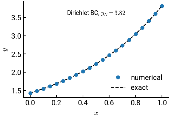
# plot the result
fig, ax = plt.subplots()
ax.plot(x, y, 'o', label='numerical')
ax.plot(x1, y_exact, 'k--', lw=2, label='exact', zorder=-5)
ax.set(xlabel='$x$', ylabel='$y$')
ax.annotate("Dirichlet BC, $y_N = 3.82$", (0.5, 3.57), ha='center', fontsize=14)
ax.legend()
plt.show()