Example 11-4: Backward Euler

Now that we’ve spent some time looking at forward Euler, it’s time to introduce backward Euler. This algorithm is essentially the same as forward Euler, but now \(y_{n+1}\) appears on both sides of the finite difference approximation. As such, this falls under the class of implicit schemes.

Summary of commands

No new commands are demonstrated in this exercise.

Backward Euler demo

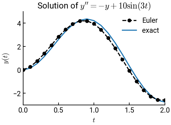
Consider the same IVP that we saw in Example 11-12:

\[ y' = -y + 10 \sin(3t), \quad y(0) = 0, \quad 0 \le t \le 2 \]

The exact solution is \(y = -3 \cos (3t) + \sin (3t) + 3e^{-t}\).

We’ll numerically solve this ODE using backward Euler and a step size of \(h = 0.1\).

# import libraries
import numpy as np
import matplotlib.pyplot as plt

# initialization
h = 0.1
t0 = 0
tf = 2
y0 = 0
y = [y0]
t = [t0]

# backward Euler loop
n = 0
while t[n] < tf:
    t.append(t[n] + h)
    y.append((y[n] + 10 * h * np.sin(3 * t[n + 1])) / (1 + h))
    n += 1

# exact solution
t = np.array(t)
y_exact = -3 * np.cos(3 * t) + np.sin(3 * t) + 3 * np.exp(-t)

# plot result
fig, ax = plt.subplots()
ax.plot(t, y, 'k--o', lw=2.5, label='Euler')
ax.plot(t, y_exact, lw=2.5, label='exact', zorder=-5)
ax.set(xlabel='$t$', ylabel='$y(t)$', title=r"Solution of $y'' = -y + 10 \sin(3t)$",
       xlim=[0, tf], ylim=[-3, 5])
ax.legend()
plt.show()