Example 11-3: Logistic function#
We will provide another demonstration of Euler’s method, and this time, we will build on the previous example by also writing a standalone function for Euler’s method. The advantage of this structure is that the function for Euler’s method becomes generic and can be reused for any ODE function \(f(t, y)\).
Summary of commands#
In this exercise, we will demonstrate the following:
Writing our own function in Python.
Having functions as the input arguments to other functions.
The second point is especially cool. The syntax might look something like this:
def outer_function(f, a, b):
    ans = f(a, b)    # note this!
    return ans

def input_function(c, d):
    return 2 * c  + d

# calling it
outer_function(input_function, 1, 2)
Euler’s method with standalone function#
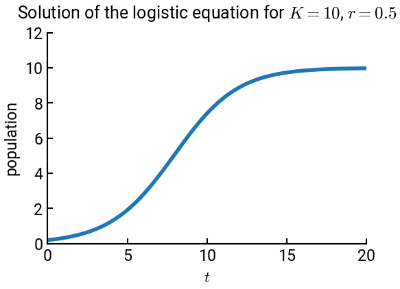
Consider the logistic equation we’ve previously seen:
where the intrinsic growth rate \(r\) and the carrying capacity \(K\) are selected to be \(r = 0.5\) and \(K = 10\). The initial population is \(y_0 = 0.2\). We will solve this ODE for the range \(0 \le t \le 20\).
Before we write our standalone Euler’s method function, we’ll sketch the ideas using pseudocode (generally helpful!)
def my_euler(input_args):
    create array of time values from t0 to tf, spaced by h
    initialize y array with y0
    set counter n = 1
    until tf is reached, loop:
        update y based on h * first_derivative_function
        increment counter n by 1
    return the time and y arrays
Writing pseudocode can help us validate our logic for consistency without being limited by the syntax of Python.
We can also anticipate the input arguments we need; in particular, we see where our custom ODE function plugs into the first_derivative_function above.
Below we give the solution first using a while loop.
# import libraries
import numpy as np
import matplotlib.pyplot as plt

# logistic function
def logistic(t, y):
    K = 10
    r = 0.5
    return r * y * (1 - y/K)

# Euler's method function
def my_euler(f, t0, tf, y0, h):
    t = np.arange(t0, tf+h, h)
    y = [y0]
    n = 0
    while t[n] < tf:
        y.append(y[n] + h * f(t[n], y[n]))
        n += 1
    return t, np.array(y)    # convert y to NumPy array for consistency

# initialize
y0 = 0.2
t0 = 0
tf = 20
h = 0.1

# execute the Euler method solver
t, y = my_euler(logistic, t0, tf, y0, h)

# plot the result
fig, ax = plt.subplots()
ax.plot(t, y)
ax.set(xlabel='$t$', ylabel='population', xlim=[0, tf], ylim=[0, 12])
ax.set_title(r"Solution of the logistic equation for $K = 10$, $r = 0.5$", fontsize=18, pad=15)
plt.show()
We could, of course, just as easily have done the same with a for loop in my_euler().
# Euler's method function
def my_euler_for(f, t0, tf, y0, h):
    t = np.arange(t0, tf+h, h)
    y = [y0]
    for n in range(len(t) - 1):
        y.append(y[n] + h * f(t[n], y[n]))
    return t, np.array(y)    # convert y to NumPy array for consistency

# execute the Euler method solver
t, y = my_euler_for(logistic, t0, tf, y0, h)

# plot the result
fig, ax = plt.subplots()
ax.plot(t, y)
ax.set(xlabel='$t$', ylabel='population', xlim=[0, tf], ylim=[0, 12])
ax.set_title(r"Solution of the logistic equation for $K = 10$, $r = 0.5$", fontsize=18, pad=15)
plt.show()