Example 12-2: Neumann boundary conditions

In Example 12-1, we worked with Dirichlet boundary conditions where the function value was fixed at the ends. Here we will work with Neumann boundary conditions, where the value of the first derivative (slope) is fixed at one of the ends.

Summary of commands

No new commands are demonstrated in this exercise as it will closely mirror Example 12-1.

Direct methods

We now rework the ODE in the previous example, but the boundary conditions are

The boundary conditions are

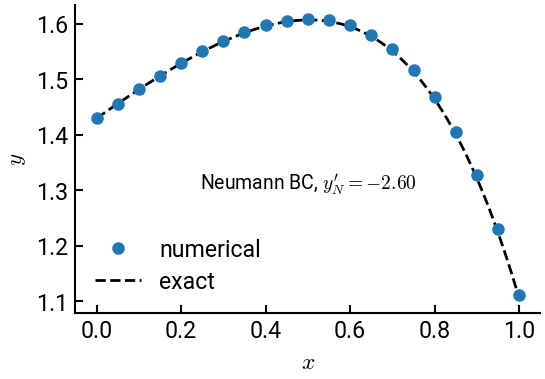
\[ y(x_L) = y_L = 1.43 \quad \text{and} \quad y'(x_R) = y_R' = -2.6 \]

and the associated coefficients are:

\[\begin{split} \begin{align} a_j &= 1 + \frac{3h}{2} \\ a_N &= 2 \\ b_j &= 2h^2 - 2 \\ c_j &= 1 - \frac{3h}{2} \\ c_N &= 0 \tag{not used} \end{align} \end{split}\]

and

\[\begin{split} \begin{align} f_2 &= h^2 \cos(x_2) - \left(1 + \frac{3h}{2} \right) y_L \\ f_j &= h^2 \cos(x_j) \\ f_{N} &= h^2 \cos(x_{N}) - 2h \left( 1 - \frac{3h}{2} \right) y_R' \end{align} \end{split}\]

# import libraries
import numpy as np
import matplotlib.pyplot as plt

# helper function to make tridiagonal matrices
def make_tridiag(a, b, c):
    """ For convenience, a, b, c should all be the same length.
        The function will automatically subset and place on the 
        corresponding diagonal. """
    return np.diag(a[1:], -1) + np.diag(b, 0) + np.diag(c[:-1], 1)

# constants
N = 21
yL = 1.43
ypR = -2.6
xL = 0
xR = 1
h = (xR - xL) / (N - 1)
x = np.linspace(xL, xR, N)

# construct matrix - carefully check dimensions and indices!!
a = np.ones(N - 1) * 1 + 3 * h / 2
a[-1] = 2
b = np.ones(N - 1) * 2 * h**2 - 2
c = np.ones(N - 1) * 1 - 3 * h / 2
A = make_tridiag(a, b, c)

# construct f and solve
f = np.cos(x[1:]) * h**2
f[0] -= (1 + 3 * h / 2) * yL
f[-1] -= 2 * h * (1 - 3 * h / 2) * ypR
y = np.linalg.solve(A, f)
y = np.concatenate([[yL], y])   # only need to add left BC this time

# exact solution
x1 = np.linspace(xL, xR, 10000)
y_exact = 1.8250 * np.exp(x1) - 0.4950 * np.exp(2 * x1) - 3/10 * np.sin(x1) + 1/10 * np.cos(x1)

# plot the result
fig, ax = plt.subplots()
ax.plot(x, y, 'o', label='numerical')
ax.plot(x1, y_exact, 'k--', lw=2, label='exact', zorder=-1)
ax.set(xlabel='$x$', ylabel='$y$')
ax.annotate("Neumann BC, $y_N' = -2.60$", (0.5, 1.3), ha='center', fontsize=14)
ax.legend()
plt.show()