Example 12-5: Shooting method

In this final example, we’re going to move away from direct methods and discuss a different class of algorithms known as the shooting method. Now we might know our target value (e.g., if we’re launching a projectile), but for some reason our ODE system is underspecified. Therefore, we have to make iterative guesses at our boundary conditions and check to see how close we get.

Summary of commands

• We’ll be using the break keyword to exit the loop when our tolerance is reached. See the course notes for the theory behind the shooting method.

• Otherwise, we’ll be using a lot of the same machinery as previous examples.

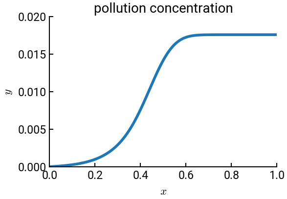
Modeling chemical pollution

Consider a river being polluted by a chemical plant. The river flow has a velocity \(V\) in the \(x\)-direction. Chemical plants along the river release toxic waste into it, modeled by the function \(S(x)\). Given that the diffusion coefficient of the toxic waste in water is \(D\), the equation governing the distribution of waste along the river is the convection diffusion equation:

\[ V \frac{dy}{dx} - D \frac{d^2y}{dx^2} = S(x) \]

where \(y(x)\) is the concentration of the toxic waste in the river. The domain is non-dimensionalized so that the total river section under consideration is \(1\), i.e., \(x = [0, 1]\), with \(x = 0\) corresponding to a point upstream of the chemical plant and \(x = 1\) a point downstream. We are asked to solve for \(y(x)\) given the following information:

\[ V = 1.0, \quad D = 0.1, \quad S(x) = 0.1 \exp \left[ -100 (x - 0.5)^2 \right] \]

and the boundary conditions

\[ y(x = 0) = 0,\ \quad \frac{dy}{dx} \bigg|_{x=1} = 0 \]

We convert this 2nd-order ODE to a system of 2 first-order ODEs with \(y_1(x) = y(x)\) and \(y_2(x) = y'(x)\). This gives us

\[\begin{split} \begin{align} y_1' &= y_2 \\ y_2' &= \frac{V}{D} y_2 - \frac{0.1}{D} \exp \left[-100(x -0.5)^2 \right] \end{align} \end{split}\]

with boundary conditions

\[ y_1(0) = 0,\ \quad y_2(1) = 0 \]

# import libraries
import numpy as np
import matplotlib.pyplot as plt

# user-defined function
def pollution(x, y, A1, A2):
    S = 0.1 * np.exp(-100 * (x - 0.5)**2)
    return np.array([y[1], A1/A2 * y[1] - S/A2])

# 4th-order Runge-Kutta
def RK4(f, t0, tf, y0, h, args):
    t = np.arange(t0, tf+h, h)
    y = np.zeros((len(t), len(y0)))
    y[0, :] = y0
    for n in range(len(t) - 1):
        k1 = f(t[n], y[n, :], *args)
        k2 = f(t[n] + 0.5 * h, y[n, :] + 0.5 * h * k1, *args)
        k3 = f(t[n] + 0.5 * h, y[n, :] + 0.5 * h * k2, *args)
        k4 = f(t[n] + h, y[n, :] + h * k3, *args)
        y[n+1, :] = y[n, :] + 1/6 * h * (k1 + 2 * k2 + 2 * k3 + k4)
    return t, y

# constants
V = 1
D = 0.1
xL = 0
xR = 1
y0 = 0
yp1 = 0
target = yp1 

# initial guess
guess = [0.0, 0.005]
tol = 1e-5 
N = 1025
h = (xR - xL) / (N - 1)

print("Iteration     y''(0)      y''(1)   ")
result = []
for k in range(15):
    x, y = RK4(pollution, xL, xR, [y0, guess[k]], h, [V, D])   # solve for current guess
    result.append(y[-1, 1])                                    # store the result
    print(f"{k} {guess[k]:18.8f} {result[k]:11.6f}")

    if k > 0:
        if abs(result[k] - target) > tol:        # check for convergence
            slope = (guess[k] - guess[k-1]) / (result[k] - result[k-1])
            guess.append(guess[k-1] + slope * (target - result[k-1]))  # next guess
        else:
            break      # tolerance is reached, exit loop

# plot the results
fig, ax = plt.subplots()
ax.plot(x, y[:, 0], label='numerical')
ax.set(xlabel="$x$", ylabel="$y$", xlim=[0,1], ylim=[0, 0.02], 
       title="pollution concentration")
plt.show()

Iteration     y''(0)      y''(1)   
0         0.00000000  -33.776992
1         0.00500000   76.355337
2         0.00153347    0.000000