Example 11-1: Euler’s method#
Important!
If you’re completely new to Python, you may want to go through the exercises in the Python fundamentals notebook first!
Note
Click the and open this notebook in Colab to enable interactivity.
Note
To save your progress, make a copy of this notebook in Colab File > Save a copy in Drive and you’ll find it in My Drive > Colab Notebooks.
We will now demonstrate how to implement numerically one of the simplest methods used to solve initial value problems (IVPs) for ODEs: Euler’s method.
We will demonstrate this using both while and for loops so you can see the different syntax.
Summary of commands#
In this exercise, we will demonstrate the following:
whileloops andforloops to automate repetitive tasks.The
appendmethod for adding objects to the end of a list.
Euler’s method#
We saw that for ODEs that can be expressed in the form \(\dfrac{dy}{dt} = f(t,y)\), we can linearize the equation to obtain
which allows us to iteratively solve for \(y(t)\) by making better and better approximations in succession, indexed by \(n\). This technique is known as Euler’s method, or the forward Euler’s method more specifically. Since we are cycling through a sequence of indices \(n\), this calls for loops!
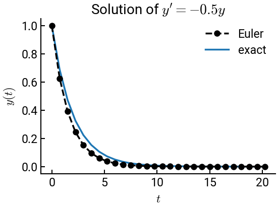
We will demonstrate this by solving the following ODE using Euler’s method:
The exact solution to this ODE is \(y = e^{-0.5 t}\).
while loop#
The trick to using a while loop is to keep an index variable (n below) and use this index to access an updated value each iteration of the loop.
We have to make sure to increment the variable or else we’ll get stuck in an infinite loop!
Note also that NumPy arrays are not dynamically (re)allocated, which means you can’t change their dimensions once created (unlike in MATLAB).
Since we may not know how many iterations we’ll be in the while loop, it doesn’t make sense to intialize t and y as arrays.
Instead, we are just going to use regular list objects from Python to store the values, starting with the initial conditions for \(t\) and \(y\).
In some cases it can be helpful to convert the list into a NumPy array using the np.array(x) constructor once we’re all done, but it is not necessary here.
# import libraries
import numpy as np
import matplotlib.pyplot as plt

# initialize
h = 0.75
t0 = 0
tf = 20
y0 = 1
y = [y0]    # initial condition stored in lists
t = [t0]    # initial condition stored in lists

# Euler while loop
n = 0
while t[n] < tf:
    t.append(t[n] + h)                 # increment t
    y.append(y[n] - 0.5 * h * y[n])    # increment y
    n += 1

# plot and compare with exact
fig, ax = plt.subplots()
ax.plot(t, y, 'k--o', lw=2.5, label='Euler')
ax.plot(t, np.exp(-0.5 * np.array(t)), lw=2.5, zorder=-5, label='exact')
ax.set(xlabel='$t$', ylabel='$y(t)$', title="Solution of $y' = -0.5 y$")
ax.legend()
plt.show()
for loop#
You will observe that, structurally, much of the code is the same.
But now, we can create the time array before the loop, since we know the exact endpoints and increment.
This also makes it easier to construct the loop, as we only have to worry about \(y\) and the index n is automatically incremented.
Remember that, generally speaking, if you know the number of iterations a process will take, it is advantageous to use a for loop.
# import libraries
import numpy as np
import matplotlib.pyplot as plt

# initialize
h = 0.75
t0 = 0
tf = 20
y0 = 1
y = [y0]
t = np.arange(t0, tf+h, h)            # preallocate, including tf

for n in range(len(t) - 1):
    y.append(y[n] - 0.5 * h * y[n])   # only update y in loop

# plot and compare with exact
fig, ax = plt.subplots()
ax.plot(t, y, 'k--o', lw=2.5, label='Euler')
ax.plot(t, np.exp(-0.5 * np.array(t)), lw=2.5, zorder=-5, label='exact')
ax.set(xlabel='$t$', ylabel='$y(t)$', title="Solution of $y' = -0.5 y$")
ax.legend()
plt.show()
Some plotting tips:
The
lwparameter is short for “line width,” helping ensure things are visible.The
zorderparameter controls the order of objects on the plot. Since \(y_{\mathrm{exact}}\) was plotted second, it would normally appear on top; but since we’re more interested in the numerical solution, we make thezorderof the second plot a decent negative number to force it to be below the numerical (black) curve.