Example 11-7: Heun’s method

Since both forward and backward Euler methods are only first-order accurate, we seek a way to improve the accuracy by combining the two by averaging them. Thus begins our exploration of multi-stage algorithms that can achieve higher orders of accuracy.

Summary of commands

No new commands are demonstrated in this exercise, but we will revisit many of the concepts from Example 11-3 to build Heun’s method.

Heun’s method

The general idea of Heun’s method (also known as “improved Euler’s method” or “two-stage Runge-Kutta”) is to perform the update in two stages:

\[\begin{split} \begin{align} k_1 &= f(t_n, y_n) \\ k_2 &= f(t_n + h, y_n + hk_1) \\ y_{n+1} &= y_n + h \left( \frac{1}{2} k_1 + \frac{1}{2} k_2 \right) \end{align} \end{split}\]

---

Now, consider the same IVP that we saw previously:

\[ y' = -y + 10 \sin(3t), \quad y(0) = 0, \quad 0 \le t \le 2 \]

We will use Heun’s method to solve the ODE using a step size of \(h = 0.1\).

# import libraries
import numpy as np
import matplotlib.pyplot as plt

# Heun's method function
def heun(f, t0, tf, y0, h):
    y = [y0]
    t = np.arange(t0, tf+h, h)
    for n in range(len(t) - 1):
        k1 = f(t[n], y[n])
        k2 = f(t[n] + h, y[n] + h * k1)
        y.append(y[n] + 0.5 * h * (k1 + k2))
    return t, np.array(y)

# logistic function
def my_func(t, y):
    return -y + 10 * np.sin(3 * t)

# initialize
y0 = 0
t0 = 0
tf = 2
h = 0.1

# execute the Euler method solver
t, y = heun(my_func, t0, tf, y0, h)
y_exact = -3 * np.cos(3 * t) + np.sin(3 * t) + 3 * np.exp(-t)

# plot the result
fig, ax = plt.subplots()
ax.plot(t, y, 'k--o', lw=2.5, label='Heun')
ax.plot(t, y_exact, lw=2.5, label='exact', zorder=-5)
ax.set(xlabel='$t$', ylabel='$y(t)$', title=r"Solution of $y'' = -y + 10 \sin(3t)$",
       xlim=[0, tf], ylim=[-3, 5])
ax.legend()
plt.show()

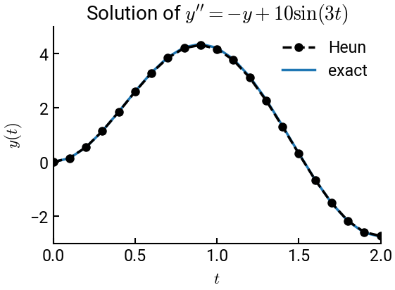
From which we can immediately see that Heun’s algorithm produces much more accurate results than either of the two Euler algorithms.