Example 11-10: Runge-Kutta for a system of ODEs

So far, we’ve explored a variety of numerical methods for solving a single ODE. Now we will extend these methods to solve a system of ODEs. You’ll see that the logic is largely the same, but we have to be more careful about indexing as \(y\) will now be a 2D array.

Summary of commands

No new commands are demonstrated in this exercise, but we will extend Example 11-8 to work for multiple dependent variables (\(y\)).

Lotka-Volterra model

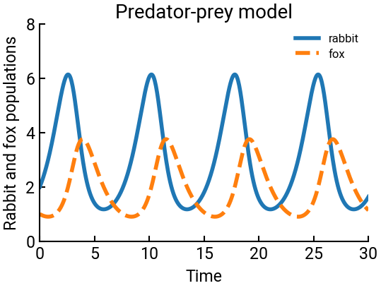
One of the best-known coupled ODEs is the Lotka-Volterra population model:

\[\begin{split} \begin{align*} \frac{dR(t)}{dt} &= aR(t) - bR(t) F(t) \\ \frac{dF(t)}{dt} &= -cF(t) + dR(t) F(t) \end{align*} \end{split}\]

where \(F(t)\) represents the population of foxes (predators) over time and \(R(t)\) represents the population of rabbits (prey). The product of the two variables represents direct interactions and \(a\), \(b\), \(c\), and \(d\) are proportionality constants.

If we put the populations into an array, we might get something like the following:

\[\begin{split} \begin{bmatrix} y(0, 0) & y(0, 1) \\ y(1, 0) & y(1, 1) \\ \vdots & \vdots \\ y(N-1, 0) & y(N-1, 1) \\ \end{bmatrix} \end{split}\]

where \(y(:, 0) = R(t)\) and \(y(:, 1) = F(t)\).

# import libraries
import numpy as np
import matplotlib.pyplot as plt

# Lotka-Volterra model
def LV(t, y, a, b, c, d):
    R, F = y    # for readability, extract the columns of y into separate variables
    return np.array([a * R - b * R * F, -c * F + d * R * F])

# 4th-order Runge-Kutta
def RK4(f, t0, tf, y0, h, args):
    t = np.arange(t0, tf + h, h)
    y = np.zeros([len(t), len(y0)])   # note!
    y[0, :] = y0    # initial condition is first row
    for n in range(len(t) - 1):
        k1 = f(t[n], y[n, :], *args)
        k2 = f(t[n] + 0.5 * h, y[n, :] + 0.5 * h * k1, *args)
        k3 = f(t[n] + 0.5 * h, y[n, :] + 0.5 * h * k2, *args)
        k4 = f(t[n] + h, y[n, :] + h * k3, *args)
        y[n+1, :] = y[n, :] + 1/6 * h * (k1 + 2 * k2 + 2 * k3 + k4)
    return t, y

# initialization
a = 1
b = 0.5
c = 0.75
d = 0.25
R0 = 2
F0 = 1
t0 = 0
tf = 30
h = 0.05

# Runge-Kutta method
t, y = RK4(LV, t0, tf, [R0, F0], h, [a, b, c, d])

# plot results
fig, ax = plt.subplots()
ax.plot(t, y[:, 0], label='rabbit')
ax.plot(t, y[:, 1], '--', label='fox')
ax.set(xlabel='Time', ylabel='Rabbit and fox populations', title="Predator-prey model",
       xlim=[0, tf], ylim=[0, 8])
ax.legend(fontsize=12)
plt.show()