9. 2D Laplace equation

When studying equilibrium properties in engineering, you’ll likely come across the Laplace equation. This relies on calculating the Laplacian, which you learned in CME 100 as \(\nabla^2 \stackrel{\text{def}}{=} \dfrac{\partial^2}{\partial x^2} + \dfrac{\partial^2}{\partial y^2} + \dfrac{\partial^2}{\partial z^2}\). In this example, we will use it to model the steady-state temperature distribution in 2D, which can be solved using Fourier series and visualized.

Summary of commands

In this exercise, we will demonstrate the following:

• np.sinh(x) - Calculate the hyperbolic sine of x.

• np.meshgrid(x, y) - Create a 2D grid of coordinate values based on 1D x and y arrays.

  • The result is two X and Y 2D arrays with the corresponding 1D arrays tiled across the other dimension.

• ax.pcolormesh(X, Y, C) - Create a pseudocolor plot of C values on a grid defined by (X, Y).

• fig.colorbar(obj) - Add a color bar corresponding to the obj plot element.

Demo

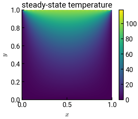
A rectangular plate is bounded by

\[\begin{split} \begin{alignat}{2} x &= 0, \quad x &&= 1 \\ y &= 0, \quad y &&= 1 \end{alignat} \end{split}\]

with the following boundary conditions:

\[\begin{split} \begin{alignat}{2} T(x, 0) &= 0, \quad T(1, y) &&= 0 \\ T(0, y) &= 0, \quad T(x, 1) &&= 100 \end{alignat} \end{split}\]

The steady-state temperature distribution is governed by \(\dfrac{\partial^2 T}{\partial x^2} + \dfrac{\partial^2 T}{\partial y^2} = 0\). The solution is:

\[ T(x,y) = \sum_{n=\text{odd}}^{\infty} \dfrac{400}{n \pi \sinh(n \pi)} \sin(n\pi x) \sinh(n \pi y)\]

Plot this temperature distribution.

# import libraries
import numpy as np
import matplotlib.pyplot as plt

# create grid
x = np.linspace(0, 1, 1000)
X, Y = np.meshgrid(x, x)
nmax = 40

# Fourier series
T = np.zeros(X.shape)
for n in np.arange(1, nmax, 2):
    Bn = 400 / (n * np.pi * np.sinh(n * np.pi))
    T += Bn * np.sin(n * np.pi * X) * np.sinh(n * np.pi * Y)

fig, ax = plt.subplots()
im = ax.pcolormesh(X, Y, T)
# im = ax.imshow(T, origin='lower')   # multiple ways to solve a problem!
plt.colorbar(im)
ax.set(xlabel="$x$", ylabel="$y$", title="steady-state temperature", aspect='equal')
plt.show()

Tip

By default, Python 2D arrays have \((0,0)\) in the upper-left corner. In ax.imshow(), we can explicitly pass the origin parameter to change the origin to the lower-left corner.