12. 2D Laplace equation using iterative methods

In Exercise 9, we solved the 2D Laplace equation for the steady-state heat distribution using Fourier series. Now, we will show how you can solve the Laplace equation using iterative schemes such as the Jacobi method and Gauss-Seidel method.

Summary of commands

In this exercise, we will demonstrate the following:

• np.meshgrid(x, y) and ax.pcolormesh(X, Y, C), as we saw in Exercise 9.

• using a while loop to iterate until convergence.

Demo

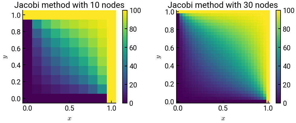
A square cooling plate of length \(1\) is maintained at \(0\) °C. When the machine turns on, two sides are heated to \(100\) °C, as shown in the figure. Using \(10\) nodes and \(30\) nodes, use the Jacobi iteration method to plot the steady-state temperature after the machine turns on, to within a \(1\%\) error. The iteration scheme is

\[ u_{i,j}^{n+1} = \dfrac{u_{i-1,j}^{n} + u_{i+1,j}^{n} + u_{i,j-1}^{n} + u_{i,j+1}^{n}}{4} \]

# import libraries
import numpy as np
import matplotlib.pyplot as plt

fig, ax = plt.subplots(ncols=2, figsize=(12, 4))
for k,nodes in enumerate([10, 30]):
    # initialize
    M = nodes
    N = nodes
    u = np.zeros((M, N))
    u[-1, :] = 100
    u[:, -1] = 100

    # loop until convergence
    error = 1
    while error > 0.01:
        u_old = u.copy()    # make a copy of the old array
        for i in range(1, M-1):
            for j in range(1, N-1):
                # Jacobi updates
                u[i,j] = (u_old[i-1,j] + u_old[i+1,j] + u_old[i,j-1] + u_old[i,j+1])/4
        error = np.max(np.abs(u_old - u))

    # make a plot of the grid
    X, Y = np.meshgrid(np.linspace(0, 1, nodes), np.linspace(0, 1, nodes))
    h = ax[k].pcolormesh(X, Y, u)
    fig.colorbar(h)
    ax[k].set(xlabel='$x$', ylabel='$y$', aspect='equal',
              title=f"Jacobi method with {N} nodes")
plt.show()

Note

Here we made the choice for the number of nodes quite evident in the shading. Of course, there are ways to be clever, such as adding shading='gouraud' into ax.pcolormesh() to make the plots look smoother and nearly identical!