6. Fourier series

Fourier series is a powerful technique that uses a summation of trigonometric functions (i.e., sines and cosines) to approximate periodic functions and solve differential equations. In this section of the workbook, we’ll look at how we can construct numerical Fourier series to solve a variety of different problems.

Summary of commands

In this exercise, we will demonstrate the following:

• np.zeros(shape) - Function for constructing a \(0\)-matrix of the required shape.

  • If you have an existing array M and you want a \(0\)-matrix of the same dimensions, using M.shape for the argument of this function.

• for i,x in enumerate(X) - Loop through the elements of array X, but return the associated index i along with each element x.

Demo

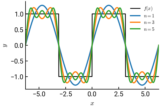
For the function

\[\begin{split} f(x) = \begin{cases} -1 & -\pi < x < 0 \\ 1 & 0 < x < \pi \end{cases}, \end{split}\]

the odd Fourier expansion is given by

\[ f(x) = \sum_{n = \text{odd}}^{\infty} \dfrac{4}{n\pi} \sin(nx) \]

Plot the actual function and the first \(3\) partial sums over the domain \(-2\pi < x < 2\pi\), all on the same set of axes. Observe how the Fourier series is accurate over many periods.

# import libraries
import numpy as np
import matplotlib.pyplot as plt

# initialize arrays
x = np.linspace(-2*np.pi, 2*np.pi, 1000)
y = np.zeros(x.shape)
for i,xx in enumerate(x):
    if xx <= -np.pi or (xx > 0 and xx < np.pi):
        y[i] = 1
    else:
        y[i] = -1

# create the figure and plot exact function
fig, ax = plt.subplots()
ax.plot(x, y, 'k-', lw=2, label="$f(x)$")

# construct the Fourier series
A0 = 0
y = A0
for n in range(1, 6, 2):    # remember the upper limit is not included, use 6 not 5
    An = 0
    Bn = 4 / (n * np.pi)
    y += An * np.cos(n * x) + Bn * np.sin(n * x)   # splitting it like this is cleaner
    ax.plot(x, y, lw=3, label=f"$n = {n}$")

ax.set(xlabel='$x$', ylabel='$y$', xlim=[-2*np.pi,2*np.pi])
ax.legend(fontsize=12)
plt.show()