14. Time-dependent heat equation - Implicit scheme

For this final exercise, we will redo the previous example with the heat equation, but this time we will use an implicit scheme. Recall this means that unknown values at time step \(t^{n + 1}\) are included in the equations to be solved at time step \(t^n\). While this is computationally more expensive as it involves solving a matrix equation at each step, it grants better numerical stability, potentially allowing you to use a larger time step. Let’s see how we can use Python to do this.

Summary of commands

In this exercise, we will apply several of the commands we’ve already learned!

Demo

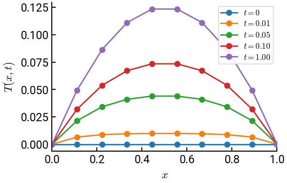
Heat generated from an electric wire is defined by the time-dependent heat equation:

\[ \lambda^2 \dfrac{\partial^2 u}{\partial x^2} + q = \dfrac{\partial u}{\partial t} \]

with \(u(0,t) = u(L,t) = 0\) and \(u(x,0) = 0\).

Use the fully implicit discretization scheme with \(N = 10\), \(L = 1\), \(\lambda = 1\), and \(q = 1\) to find the temperature distribution at \(t = \begin{bmatrix} 0 & 0.01 & 0.05 & 0.1 & 1 \end{bmatrix}\). Take \(dt = 0.01\).

Note: The fully implicit distribution scheme is \(\lambda^2 \dfrac{u_{i-1}^{n+1} - 2u_i^{n+1} + u_{i+1}^{n+1}}{\Delta x^2} + q = \dfrac{u_{i}^{n+1} - u_i^n}{\Delta t}\).

# import libraries
import numpy as np
import matplotlib.pyplot as plt

# helper function to make tridiagonal matrices
def make_tridiag(a, b, c):
    return np.diag(a[1:], -1) + np.diag(b, 0) + np.diag(c[:-1], 1)
    
# constants
N = 10
L = 1
h = L/(N-1)
lamda = 1
q = 1
dt = 0.01

# initialize A
r = lamda**2 * dt / h**2
A = make_tridiag(-r * np.ones(N-2), (1 + 2*r) * np.ones(N-2), -r * np.ones(N-2))
b = q * dt * np.ones(N-2)

# initialize solution
t = np.array([0, 0.01, 0.05, 0.1, 1])
x = np.linspace(0, L, N)
u = np.zeros(N)

# plot initial condition
fig, ax = plt.subplots()
ax.plot(x, u, 'o-', lw=2, label="$t = 0$")
ax.set(xlabel='$x$', ylabel="$T(x,t)$", xlim=[0,1])

# solve
for j in range(1, int(t[-1]/dt)+1):
    u[1:-1] = np.linalg.solve(A, b + u[1:-1])
    if j * dt in t:
        ax.plot(x, u, 'o-', lw=2, label=f"$t = {j * dt:.2f}$")

ax.legend(fontsize=12, framealpha=0.9)
plt.show()