3. Least squares regression

In science and engineering, it is common practice to fit a model to experimental data. But how do you pick a good model, or determine if your model is good enough? One idea could be this: If your model has parameters, then you pick the parameters that result in a model whose predictions give the “lowest error” when validated against the existing data. If the “lowest error” is computed as the mean squared error, then you get the least squares regression algorithm (regression because we’re modeling a quantitative metric). Let’s how Python can help us compute the least squares regression line, otherwise known as the line of best fit.

Summary of commands

In this exercise, we will demonstrate the following:

• np.polyfit(x, y, deg) - Finds the coefficients of a polynomial of degree deg to fit the data (x, y) by minimizing the least squares error. Note the resulting vector, call it p, contains the coefficients of the polynomial in decreasing order of \(x\).

• np.polyval(p, x) - Evaluates a fitted polynomial with coefficients p on new input values x.

Demo

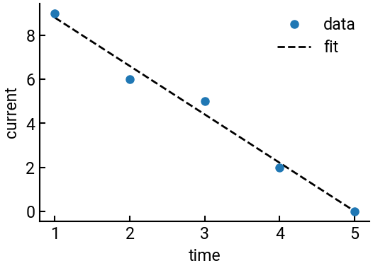
Data from a current flowing across a capacitor is recorded as \((t,I)\) pairs. If the theoretical decrease in current is supposed to be linear, plot the graph that best represents the data: \((1,9)\), \((2,6)\), \((3,5)\), \((4,2)\), and \((5,0)\).

# import libraries
import numpy as np
import matplotlib.pyplot as plt

# initialize data
t = np.array([1, 2, 3, 4, 5])
I = np.array([9, 6, 5, 2, 0])

# fit a linear polynomial
p = np.polyfit(t, I, 1)   # third arg is degree of polynomial = 1
Ifit = np.polyval(p, t)   # evaluate the polynomial

# make the plot
fig, ax = plt.subplots()
ax.plot(t, I, 'o', label='data')
ax.plot(t, Ifit, 'k--', lw=2, label='fit', zorder=-5)
ax.set(xlabel='time', ylabel='current')
ax.legend()
plt.show()

Tip

• The lw parameter is short for “line width,” helping ensure things are visible.

• The zorder parameter controls the order of objects on the plot. Since Ifit was plotted second, it would normally appear on top; but since we’re more interested in the numerical solution, we make the zorder of the line a decent negative number to force it to be below the data (blue dots).