5. Regression and correlation analyses

Regression and correlation analyses are statistical techniques used to examine the relationships between variables, enabling us to understand how changes in one variable may affect another. By quantifying these relationships, we can make predictions and informed decisions based on data. Much of the advances (and hype) in the field of AI for Science rest on performing regressions and leveraging correlations!

Summary of commands

In this exercise, we will demonstrate the following:

• NumPy:

  • np.polyfit(x, y, deg) - Construct a least squares polynomial fit of y vs. x of degree deg.

  • np.corrcoef(x, y) - Calculate Pearson correlation coefficients between arrays x and y.

  • np.polyval(p, x) - Evaluate a fitted polynomial p at specific values x.

Demo

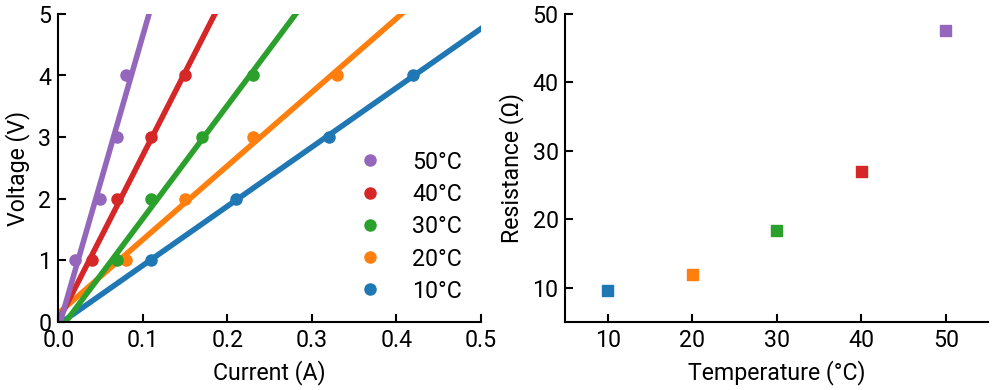
Thermistors are passive devices frequently used to measure temperature. They are resistive elements whose resistance increases as a function of temperature. To calibrate a thermistor, a voltage is applied across its terminals and the value of the current is recorded for a given temperature. The data collected is shown in the table below (current in amperes and voltage in volts).

\(T = 10 ^{\circ}\mathrm{C}\)		\(T = 20 ^{\circ}\mathrm{C}\)		\(T = 30 ^{\circ}\mathrm{C}\)		\(T = 40 ^{\circ}\mathrm{C}\)		\(T = 50 ^{\circ}\mathrm{C}\)
\(I\)	\(V\)	\(I\)	\(V\)	\(I\)	\(V\)	\(I\)	\(V\)	\(I\)	\(V\)
0.11	1	0.08	1	0.07	1	0.04	1	0.02	1
0.21	2	0.15	2	0.11	2	0.07	2	0.05	2
0.32	3	0.23	3	0.17	3	0.11	3	0.07	3
0.42	4	0.33	4	0.23	4	0.15	4	0.08	4

Part (a)

For each value of the temperature, plot on the same set of axes a linear curve fit of the voltage versus current through the thermistor and separately a calibration curve (resistance versus temperature).

Important

The coefficients that are returned from np.polyfit() always correspond to decreasing powers of \(x\). So for the function \(y = ax^2 + bx + c\), the returned coefficients \(\vec{p} = \begin{bmatrix} p_0 & p_1 & p_2 \end{bmatrix}\) correspond to \(p_0 = a\), \(p_1 = b\), and \(p_2 = c\).

Note

Notice how label= in the plotting function and ax.legend() work together to label different lines!

# import libraries
import numpy as np
import matplotlib.pyplot as plt

# data
V = np.array([1, 2, 3, 4])
I10 = np.array([0.11, 0.21, 0.32, 0.42])
I20 = np.array([0.08, 0.15, 0.23, 0.33])
I30 = np.array([0.07, 0.11, 0.17, 0.23])
I40 = np.array([0.04, 0.07, 0.11, 0.15])
I50 = np.array([0.02, 0.05, 0.07, 0.08])
T = [10, 20, 30, 40, 50]

# construct fit
p10 = np.polyfit(I10, V, 1)
p20 = np.polyfit(I20, V, 1)
p30 = np.polyfit(I30, V, 1)
p40 = np.polyfit(I40, V, 1)
p50 = np.polyfit(I50, V, 1)

# plot data
fig, (ax1, ax2) = plt.subplots(figsize=(12,4), ncols=2)   # create two axes! 
ax1.plot(I10, V, 'o', label=f'{T[0]}°C')
ax1.plot(I20, V, 'o', label=f'{T[1]}°C')
ax1.plot(I30, V, 'o', label=f'{T[2]}°C')
ax1.plot(I40, V, 'o', label=f'{T[3]}°C')
ax1.plot(I50, V, 'o', label=f'{T[4]}°C')

# calculate fit lines and plot them
x = np.linspace(0, 0.5, 100)
ax1.plot(x, np.polyval(p10, x), c='C0', zorder=-3)
ax1.plot(x, np.polyval(p20, x), c='C1', zorder=-3)
ax1.plot(x, np.polyval(p30, x), c='C2', zorder=-3)
ax1.plot(x, np.polyval(p40, x), c='C3', zorder=-3)
ax1.plot(x, np.polyval(p50, x), c='C4', zorder=-3)
ax1.legend(reverse=True)
ax1.set(xlabel='Current (A)', ylabel='Voltage (V)', xlim=[0,0.5], ylim=[0,5])

# make the resistance calibration curve - extract the slope from the fit
R = [p10[0], p20[0], p30[0], p40[0], p50[0]]
ax2.scatter(T, R, marker='s', color=[f"C{i}" for i in range(5)])
ax2.set(xlim=[5,55], ylim=[5,50], xlabel="Temperature (°C)", ylabel="Resistance (Ω)")

plt.show()

Part (b)

Compute the coefficient of determination for each of the five sets of data. Note that np.corrcoef() returns a \(m \times m\) matrix of correlation coefficients for all \(m\) variables, so we will want to select the off-diagonal terms.

rho10 = np.corrcoef(I10, V)
print(f"The coefficient of determination for 10°C is {rho10[0,1]**2:.4f}.")

rho20 = np.corrcoef(I20, V)
print(f"The coefficient of determination for 20°C is {rho20[0,1]**2:.4f}.")

rho30 = np.corrcoef(I30, V)
print(f"The coefficient of determination for 30°C is {rho30[0,1]**2:.4f}.")

rho40 = np.corrcoef(I40, V)
print(f"The coefficient of determination for 40°C is {rho40[0,1]**2:.4f}.")

rho50 = np.corrcoef(I50, V)
print(f"The coefficient of determination for 50°C is {rho50[0,1]**2:.4f}.")

The coefficient of determination for 10°C is 0.9996.
The coefficient of determination for 20°C is 0.9934.
The coefficient of determination for 30°C is 0.9918.
The coefficient of determination for 40°C is 0.9956.
The coefficient of determination for 50°C is 0.9524.