Python fundamentals#
Note
Click the and open this notebook in Colab to enable interactivity. We encourage you to experiment with customized values to deepen your learning.
Note
To save your progress, make a copy of this notebook in Colab File > Save a copy in Drive and you’ll find it in My Drive > Colab Notebooks.
In this notebook, we’ll provide a quick tutorial of Python to familiarize you with common use cases and syntax.
Contents#
1. Python as a calculator#
You can directly type numerical expressions into a code cell and execute it to run the computation.
In the example below, the asterisk * symbolizes scalar multiplication.
60 * 60 * 24 * 365
31536000
Many other operations are also possible, some have intuitive syntax, others less so.
1 + 1
2
5 / (1 + 2)
1.6666666666666667
5 // 3
1
In addition to integers (int) and floats (float, decimals), another data type you will often encounter is strings (str), which are literal expressions for text.
They can be enclosed in double " or single ' quotes, but you have to be consistent.
"Hello, World!"
'Hello, World!'
Note that in the above examples, the output automatically appeared when the cell was executed.
This will occur for the last line only, and can be suppressed with a trailing semicolon ; if so desired.
To force display of any quantity from any line, you can always use the print() function, like so:
# comments start with a pound sign and don't affect the code
print(3.1415)
print('CME 100')
3.1415
CME 100
print() is very helpful for debugging!
Feel free to experiment on your own.
The final data type we should cover is the Boolean (bool), which represents True or False.
There are a couple of ways to do this, either with a literal or an expression.
Note that in Python, to check for equality between two things uses the double equals sign (==).
A single equals sign is for assignment (below).
a = True    # assignment to a variable, see next section
print(a)
print(1 == 2)
True
False
Your turn#
In the code cell below, compute the product of all the integers from \(1\) to \(9\).
# TODO: Write your solution below
2. General Python paradigms#
In addition to being used as a calculator, Python can store inputs or outputs into variables using the assignment operator (=).
# Define a
a = 2
print(a)
2
# Define b
b = 5
b
5
# Compute c
c = a + b ** 2   # exponentiation is two asterisks (not carat!)
print(c)
27
# Compute a different value for c
c = a + 2 * b
print(c)
12
“Restart and run all” or it didn’t happen#
With Jupyter notebooks, you have the power to run cells in any order you want. And with great power comes great responsibility. It’s easy to get variables mixed up and then your notebook starts giving you errors.
So if you ever need to reset anything, the easiest way is to go to Runtime > Restart session and run all on Colab or Run > Restart Kernel and Run All Cells... on Jupyter Lab.
This clears all variables and outputs from the workspace and runs your notebook from top to bottom.
Note
If you’re coming from MATLAB, you may be familiar with putting clear; close all; clc; at the top of your script.
This is essentially equivalent.
First, try running this following cell:
c = 2 ** 3
Before you run the next cell, try to restart the kernel by clicking Runtime > Restart session or Kernel > Restart Kernel... and then try running the next cell, which shows the variable you computed before clearing the runtime.
c
8
Data structures#
In addition to standard data types, there are data structures which are larger constructs that can store data (variables, values, etc.).
Perhaps the most common one you will use is the list, which are values within square brackets [].
See the examples below.
# creating lists
a = [1, 2, 3, 7]             # a list of integers
print(a)
b = [3, 'hi', 3.14, True]    # lists can be heterogeneous!
print(b)
c = []                       # the empty list!
print(c)
[1, 2, 3, 7]
[3, 'hi', 3.14, True]
[]
Manipulating lists#
There are so many fun things you can do with lists. Here we will only show a few.
Important
Python is 0-indexed which means the first element of my_list is my_list[0], not my_list[1]!
This is one of the biggest differences between Python and MATLAB.
# indexing into lists
a = [1, 2, 3, 4, 5, 6, 7, 8, 9]
print(a[0], a[3], a[-1])    # what's the last one doing??

# slicing a list (taking a range of values)
print(a[1:4], a[6:])       # start index is inclusive, end index is exclusive
print(a[::-1])             # ta-da!

# adding to a list with append()
a.append(42)
print(a)
1 4 9
[2, 3, 4] [7, 8, 9]
[9, 8, 7, 6, 5, 4, 3, 2, 1]
[1, 2, 3, 4, 5, 6, 7, 8, 9, 42]
There are many more data structures available to you, such as sets, dictionaries, etc. We encourage you to read more if you’re curious or as you encounter them.
Your turn#
Create a list of the first five positive integers.
Then change the third element to 7.
Print the list to confirm the change was made.
# TODO: Write your solution below
Control flow#
This is the general term used to describe constructs (often based on logical expressions) that control the order of program execution. We’ll divide this into two categories for now: conditionals and loops.
Conditional statements#
We use this to describe if, elif (short for “else if”), and else statements.
The general structure is like this:
if condition1:
    <do something only when condition1 is True>
elif condition2:
    <otherwise, do something else if condition2 is True> (and condition1 was False)
else:
    <otherwise, do something else>
Note
if is required, and the other two are optional.
Note
In MATLAB, control flow blocks have an end to conclude. No need for that in Python!
a = 2
if a == 2:
    print("a equals 2")

if a > 3:
    print("a is large")
else:
    print("a is small")
a equals 2
a is small
Take a look at this:
b = 4
if a == 2 and b == 4:
    print("wow!")
wow!
Important
In Python, logical “and” uses the actual word and instead of the symbols && as it’s commonly done in other languages.
Similarly, logical “or” uses the actual word or.
Finally, please don’t confuse these keywords (no quotes) with the literal strings 'and' and 'or'!
Loops#
There are many types of loops, which enable you to automate repetitive tasks, and they boil down to two main flavors:
forloops: When you know how many times you want something done.whileloops: When you know the stop condition (but might not know or don’t care how long it takes to get there).
The for loop syntax in Python is:
for i in collection:
    <do something repeatedly, where each iteration, the variable i takes on a different value in the collection>
where collection is usually a list-like object of values.
The for loop stops when all the items in the collection are used once.
A very common expression you’ll see for collection is range(N), which is a built-in function that enumerates numbers from 0 up to N (not inclusive).
The full function signature is range(start, stop, step), going from start to stop (not inclusive) in steps of size step.
The while loop syntax in Python is:
while condition:
    <do something repeatedly until condition becomes False>
    # Try not to get stuck in an infinite loop!
Let’s see these in action.
j = 0
for i in range(5):
    j += i
    print(i, j)

print()   # print an empty line for clarity
while j > 5:
    print(j)
    j -= 1
0 0
1 1
2 3
3 6
4 10

10
9
8
7
6
Your turn#
Loop through the first ten positive integers. Print odd numbers as they are and print the negative value for even numbers.
Hint: In Python, the modulo operator %, used as a % b, returns the remainder when \(a\) is divided by \(b\).
# TODO: Write your solution below
User-defined functions#
Sometimes, writing your own functions can be helpful for solving problems, and we will practice this in the context of applying statistical methods. In CS 106A and other contexts, this technique is called decomposition and makes your code more readable, extensible, and often more efficient.
In Python, the syntax for defining your own function is:
def my_func_name(arg1, arg2, ...):
    """ optional docstring to explain purpose, arguments, etc. """
    do something
    return something   # optional

my_func_name(args)     # calling the function
The
defat the start is required, as is the colon at the end of the first line.Just like variables, function names should be descriptive.
Arguments are optional, but you’ll probably have some input variables.
Docstrings are optional but very nice to have (for others and future you). No need though if the function is very simple.
Variables defined in the function body (including arguments) have local scope, i.e., they don’t exist outside the function.
Returning a value is generally optional, but you’ll probably have something.
Calling the function works as with any other built-in function.
Below we give a short example:
def square_input(x):
    """ Takes an input and squares it. """
    local_scope = 0
    return x ** 2

print(square_input(5))
print(local_scope)    # errors!
25
---------------------------------------------------------------------------
NameError                                 Traceback (most recent call last)
Cell In[22], line 7
      4     return x ** 2
      6 print(square_input(5))
----> 7 print(local_scope)

NameError: name 'local_scope' is not defined
3. Scientific computing with NumPy#
Now that we’re familiar with native Python, it’s time to explore what it can accomplish for scientific computing. In engineering mathematics, we often have to work with vector quantities, like force, position, electric field, etc. In scientific computing in Python, these vectors are encoded as one-dimensional NumPy arrays, and these exercises walk you through how to create them, starting from the lists that you’ve already seen.
my_list = [1, 2, 3]

print(type(my_list))   # function that shows the class of an object
print(my_list)
<class 'list'>
[1, 2, 3]
Now, the above looks like a vector, but we’re not quite there yet. We have to convert it to an array using the canonical scientific computing library NumPy.
Like other programming languages (including MATLAB), in Python we have to import any special packages we want to use, such as:
import my_package_name

my_package_name.special_function()
And then any functions we want to use from that package will have the package name prepended with a period. But, since NumPy is used so frequently, the community has a special paradigm to abbreviate the package import (with an alias) as follows:
import numpy as np

np.special_function()
This saves your fingers a bit, and we will adopt this practice as well.
We will import NumPy and then convert the list from above to a NumPy array using the np.array() constructor.
import numpy as np
my_array = np.array(my_list)

print(type(my_array))
print(my_array)
<class 'numpy.ndarray'>
[1 2 3]
Note how the printed array looks the same as the list, but it is a different class.
Note
We should mention: Not only do you have to import special packages, but you also have to install them into your Python environment. Luckily, if you’re using the Colab environment, all of the packages we’re using are common enough to come pre-installed.
Now we’ll do a series of tasks:
Display each element. We can select array elements by using the appropriate index,
array[ind].Multiple the first and second elements. We use the standard
*operator with the selected elements.Change the third element to
4and display the new vector on the screen.
# Display each element
print(my_array[0])
print(my_array[1])
print(my_array[2])
print()

# Multiply the first and second elements
print(my_array[0] * my_array[1])
print()

# Change the third element to 4
my_array[2] = 4
print(my_array)
1
2
3

2

[1 2 4]
2D arrays, i.e., matrices#
To create a 2D NumPy array (or \(N\)-dimensional), you can construct it from a list of lists, as follows:
import numpy as np
list2 = [ [1, 2, 3], [4, 5, 6] ]
arr = np.array(list2)
arr
array([[1, 2, 3],
       [4, 5, 6]])
Indexing into a 2D array requires commas separating the different axes (row first, then column). Recall that arrays are 0-indexed in Python!
print(arr[0, 1])
2
Helper functions#
Creating vectors manually isn’t bad when there are only a few elements, but it would be quite annoying if you had dozens or hundreds of entries. 😵💫 Luckily, there are some convenient functions that can be employed depending on your use case.
You want exactly \(N\) equally spaced values#
Here you want to use the np.linspace(start, stop, num) function, which accepts as arguments:
start: The first value of your array. Required.stop: The last value of your array. Required.num: The total number of elements in your array, equally spaced between start and stop inclusive (by default). If you do not specify this parameter, the default is50.
my_array2 = np.linspace(0, 10, 6)
print(my_array2)
[ 0. 2. 4. 6. 8. 10.]
Some notes:
In Python, functions can be called with explicit parameter names, if you want. So
np.linspace(start=0, stop=10, num=6)also would’ve worked.You can use
array.shapeto check the dimensions of the vector you constructed.array.sizereturns the total number of elements (essentially a product of all array dimensions).
Note
NumPy can be a little tricky when it comes to vectors (1-D arrays) and whether it’s a row vector or column vector.
You’ll notice the shape below is abbreviated (6,).
We’ll discuss this nuance later when we encounter it.
my_array2 = np.linspace(start=0, stop=10, num=6)
print(my_array2)
print(my_array2.shape)
print(my_array2.size)
[ 0.  2.  4.  6.  8. 10.]
(6,)
6
You want values equally spaced by \(\delta\)#
Here you want to use the np.arange(start, stop, step) function, which accepts as arguments:
start: The first value of your array. Default is0, but best to always specify.stop: The last value of your array, not inclusive. Required.step: The increment between values starting fromstartand going up to but not includingstop. Default is1.
# not quite!
my_array3 = np.arange(0, 10, 2)
print(my_array3)

# better
my_array3_redo = np.arange(0, 11, 2)
print(my_array3_redo)
[0 2 4 6 8]
[ 0  2  4  6  8 10]
Element-wise operations#
We’ll define two vectors, \(x = \begin{bmatrix} 1 & -2 & 5 & 3 \end{bmatrix}\) and \(y = \begin{bmatrix} 4 & 1 & 0 & -1 \end{bmatrix}\). We’ll multiply \(x\) and \(y\) element-by-element, and then compute the squares of the elements of \(x\). With NumPy, this is done in the ways you’d expect.
import numpy as np    # we do this every time
x = np.array([1, -2, 5, 3])
y = np.array([4, 1, 0, -1])

print("Multiplication:")
z = x * y
print(z)

print("Squaring x:")
print(x ** 2)
Multiplication:
[ 4 -2  0 -3]
Squaring x:
[ 1  4 25  9]
Note
In MATLAB, you may be used to .* and ./ to perform element-wise multiplication and division.
In NumPy, this is the default behavior.
Important
This is not what happens with lists in Python! Using the same operators could generate errors or incorrect behavior.
# create two lists
xl = [1, -2, 5, 3]
yl = [4, 1, 0, -1]
print(type(xl), xl)

# try adding them
zl = xl + yl
print(zl)

# try multiplying them
print(xl * yl)
<class 'list'> [1, -2, 5, 3]
[1, -2, 5, 3, 4, 1, 0, -1]
---------------------------------------------------------------------------
TypeError                                 Traceback (most recent call last)
Cell In[32], line 11
      8 print(zl)
     10 # try multiplying them
---> 11 print(xl * yl)

TypeError: can't multiply sequence by non-int of type 'list'
Yikes.
There are also many NumPy functions that can operate on arrays in an element-wise fashion, such as the following examples.
x = np.arange(-1, 3)
print(np.exp(x))
print(np.absolute(x))
print(np.sum(x))
[0.36787944 1.         2.71828183 7.3890561 ]
[1 0 1 2]
2
Your turn#
Compute the value of the following function of \(x\) between \(1\) and \(3\), using equally spaced points separated by \(0.2\).
# TODO: Write your solution below
4. Making plots with Matplotlib#
Visualization is an important skill for an engineer and there are many libraries in Python for doing so. We will use the foundation Matplotlib library and specifically the Pyplot package in this course. The standard syntax (best practice) for Pyplot is as follows:
import matplotlib.pyplot as plt    # import Pyplot with an alias
fig, ax = plt.subplots()           # create Figure and Axes objects
ax.plot(x, y)                      # or any other plotting function
plt.show()                         # show the figure underneath the code cell
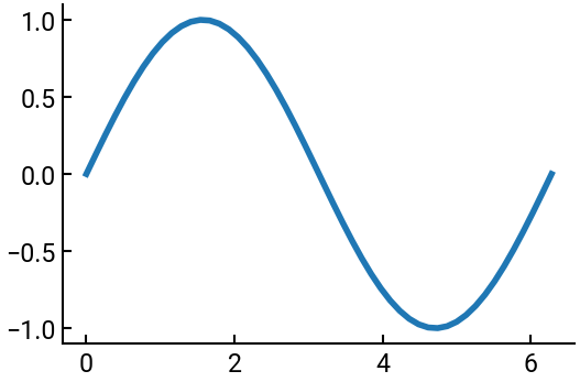
Here’s an example:
import numpy as np
import matplotlib.pyplot as plt

x = np.linspace(0, 2*np.pi)
y = np.sin(x)

fig, ax = plt.subplots()
ax.plot(x, y)
plt.show()
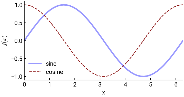
There are a ton of customizations you can apply, way more than what we can demonstrate. We’ll give a more elaborate example below, and otherwise will include links to important documentation.
Plot types - including 3D!
Setting axis features - labels, limits, titles, etc.
rcParams - the final boss
x = np.linspace(0, 2*np.pi)
y1 = np.sin(x)
y2 = np.cos(x)

fig, ax = plt.subplots(figsize=(8,4))
ax.plot(x, y1, c='blue', alpha=0.4, label='sine')
ax.plot(x, y2, c='#8C1515', ls='--', lw=2, label='cosine')
ax.set(xlabel='x', ylabel="$f(x)$", xlim=[0,2*np.pi])
ax.legend()   # note how label and legend work together!
plt.show()
Your turn#
Define and plot the function \(y(x) = |x|\) for \(x\) ranging between \(-1\) and \(1\), with \(x\) coordinates spaced by \(0.05\).
# TODO: Write your solution below
What’s next?#
So this was obviously way too quick and dense, but hopefully it gives you some foundation in Python. The best way to learn is by doing (a perk of programming—compared to other disciplines, learning is relatively low risk with rapid feedback), so we encourage you to jump right into your assignments and look stuff up as you go. If something is confusing, you can look it up on Google (some popular sites for Q&A inculde Stack Overflow, Geeks for Geeks, W3Schools) or ask generative AI.