2. Probability distributions#
Real-world processes carry uncertainty and one way to model this is with probability distributions. We’ll look at a few common probability distributions and their associated random variables as applied to engineering scenarios.
Summary of commands#
In this exercise, we will demonstrate the following:
SciPy, specifically the statistics package.
scipy.stats.binom- Binomial discrete random variable.scipy.stats.poisson- Poisson discrete random variable.scipy.stats.norm- Normal continuous random variable.
np.linspace(start, stop, num)- Returnsnumevenly spaced numbers betweenstartandstop(inclusive).
One of the nice things about using a well-written package like scipy.stats is that each of these sub-packages has standardized functions (see docs for specific input parameters):
rvs()to generate random variables. Remember this term just refers to an object that can take on a specific value from a random process (sampled from a given distribution).pmf()orpdf()to calculate the probability mass function or probability density function, respectively.cdf()to calculate the cumulative distribution function.ppf()to calculate the percent point function, which is the inverse of the CDF.
Demo#
Part (a)#
A single lot containing \(1000\) chips manufactured by a semiconductor company is known to contain \(1\%\) of defective parts. What is the probability that \(10\) parts are defective in the lot? Use both the binominal and the Poisson distributions to obtain the answer.
# import packages from SciPy library
from scipy.stats import binom, poisson

# constants
N = 1000
p = 0.01
thresh = 10

# binomial distribution
p1 = binom.pmf(thresh, N, p)
print(f"Binomial probability: {p1:.4f}")

# Poisson distribution
p2 = poisson.pmf(thresh, p*N)
print(f"Poisson probability: {p2:.4f}")
Binomial probability: 0.1257
Poisson probability: 0.1251
Note in the Poisson example we used the fact that \(\mu = pN = \lambda\) for a Poisson distribution. The similarity of the two answers demonstrates the convergence of the binomial distribution to the Poisson distribution when \(N\) is large and \(p\) is small (but non-zero).
Part (b)#
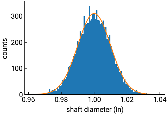
The diameters of shafts manufactured by an automotive company are normally distributed with the mean value of \(1\) inch and the standard deviation of \(0.01\) in. Each shaft is to be mounted into a bearing with an inner diameter of \(1.025\) in. Write a script to estimate the proportion of defective parts out of \(10,000\), i.e., the fraction of all parts that do not fit into the bearings. On the same set of axes plot a histogram showing the observed frequencies of the shaft diameters and the scaled density function.
# import packages from SciPy library
import numpy as np
from scipy.stats import norm
import matplotlib.pyplot as plt

# constants
N = 10000
mu = 1
sd = 0.01
thresh = 1.025

# normal distribution sampling
shafts = norm.rvs(mu, sd, N, random_state=1)   # random_state is equiv to seed for consistency
defect = sum(shafts > thresh)
print(f"Probability: {defect/N:.4f}")

# normal distribution pdf
x = np.linspace(0.96, 1.04)
y = norm.pdf(x, mu, sd)

# make the plot
fig, ax = plt.subplots()
n, b, p = ax.hist(shafts, bins=100)     # grab all three outputs: bin heights, bin positions, bin artists
ax.plot(x, y * N * (b[1]-b[0]), lw=2)   # scale the normal dist. by N * bin_width
ax.set(xlabel=r"shaft diameter (in)", ylabel='counts')
plt.show()
Probability: 0.0064
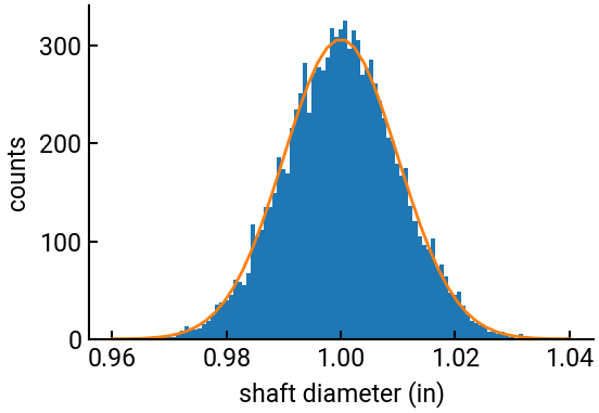
Alternatively you can use the random number generator from NumPy to sample from a normal distribution. To get the scaled density function, we use the PDF of the normal distribution:
# import packages
import numpy as np
rng = np.random.default_rng(seed=1)

# constants
N = 10000
mu = 1
sd = 0.01
thresh = 1.025

# normal distribution
shafts = rng.normal(mu, sd, N)
defect = np.sum(shafts > thresh)
print(f"Probability: {defect/N:.4f}")

# make the plot
fig, ax = plt.subplots()
n, b, p = ax.hist(shafts, bins=100)
y = 1 / (sd * np.sqrt(2 * np.pi)) * np.exp(-(b - mu)**2 / (2 * sd**2) ) * N * (b[1] - b[0])   # hack to use bin positions instead of creating new vector
ax.plot(b, y, lw=2)
ax.set(xlabel=r"shaft diameter (in)", ylabel='counts')
plt.show()
Probability: 0.0067